Note
Go to the end to download the full example code.
Multiple-kernel ridge solvers
This example demonstrates the different strategies to solve the multiple kernel ridge regression: the random search, and the hyper-gradient descent.
The random-search strategy samples some kernel weights vectors from a
Dirichlet distribution, then for each vector, it fits a KernelRidgeCV model
and computes a cross-validation score for all targets. Then it selects for each
target the kernel weight vector leading to the highest cross-validation score
(e.g. the highest R^2 value). Extensively sampling the kernel weights space
is exponentially expensive with the number of kernels, therefore this method is
computationally expensive for a large number of kernels. However, since it
reuses most of the computations for all targets, it scales very well with the
number of targets.
The hyper-gradient descent strategy takes a different route. It starts with an initial kernel weights vector per target, and updates it iteratively following the hyperparameter gradient, computed over cross-validation. As it computes a hyper-gradient descent for each target, it is more expensive computationally for large number of targets. However, the hyper-gradient descent scales very well with the number of kernels.
import numpy as np
import matplotlib.pyplot as plt

from himalaya.backend import set_backend
from himalaya.kernel_ridge import generate_dirichlet_samples

from himalaya.kernel_ridge import KernelRidgeCV
from himalaya.kernel_ridge import MultipleKernelRidgeCV
from himalaya.kernel_ridge import Kernelizer
from himalaya.kernel_ridge import ColumnKernelizer
from himalaya.utils import generate_multikernel_dataset

from sklearn.pipeline import make_pipeline
from sklearn import set_config
set_config(display='diagram')
In this example, we use the torch_cuda backend, and fit the model on GPU.
backend = set_backend("torch_cuda", on_error="warn")
/home/runner/work/himalaya/himalaya/himalaya/backend/_utils.py:66: UserWarning: Setting backend to torch_cuda failed: PyTorch with CUDA is not available..Falling back to numpy backend.
  warnings.warn(f"Setting backend to {backend} failed: {str(error)}."
Generate a random dataset
We start by generating some arbitrary scalings per kernel and targets, using samples on a Dirichlet distribution.
n_kernels = 3
n_targets = 50
n_clusters = 2
To create some clusters of weights, we take a few kernel weights samples.
kernel_weights = generate_dirichlet_samples(n_clusters, n_kernels,
                                            concentration=[.3],
                                            random_state=105)
Then, we duplicate them, and add some noise, to get clusters.
noise = 0.05
kernel_weights = backend.to_numpy(kernel_weights)
kernel_weights = np.tile(kernel_weights, (n_targets // n_clusters, 1))
kernel_weights += np.random.randn(n_targets, n_kernels) * noise

# We finish with a projection on the simplex, making kernel weights sum to one.
kernel_weights[kernel_weights < 0] = 0.
kernel_weights /= np.sum(kernel_weights, 1)[:, None]
Then, we generate a random dataset, using the arbitrary scalings.
X_train : array of shape (n_samples_train, n_features)
X_test : array of shape (n_samples_test, n_features)
Y_train : array of shape (n_samples_train, n_targets)
Y_test : array of shape (n_samples_test, n_targets)
(X_train, X_test, Y_train, Y_test,
 kernel_weights, n_features_list) = generate_multikernel_dataset(
     n_kernels=n_kernels, n_targets=n_targets, n_samples_train=600,
     n_samples_test=300, kernel_weights=kernel_weights, random_state=42)

feature_names = [f"Feature space {ii}" for ii in range(len(n_features_list))]
Define a ColumnKernelizer
We define a column kernelizer, which we will use to precompute the kernels in a pipeline.
# Find the start and end of each feature space X in Xs
start_and_end = np.concatenate([[0], np.cumsum(n_features_list)])
slices = [
    slice(start, end)
    for start, end in zip(start_and_end[:-1], start_and_end[1:])
]

kernelizers = [(name, Kernelizer(), slice_)
               for name, slice_ in zip(feature_names, slices)]
column_kernelizer = ColumnKernelizer(kernelizers)
Define the models
We define the first model, using the random search solver.
# (We pregenerate the Dirichlet random samples, to latter plot them.)
kernel_weights_sampled = generate_dirichlet_samples(n_samples=20,
                                                    n_kernels=n_kernels,
                                                    concentration=[1.],
                                                    random_state=0)

alphas = np.logspace(-10, 10, 41)
solver_params = dict(n_iter=kernel_weights_sampled, alphas=alphas,
                     n_targets_batch=200, n_alphas_batch=20,
                     n_targets_batch_refit=200, jitter_alphas=True)

model_1 = MultipleKernelRidgeCV(kernels="precomputed", solver="random_search",
                                solver_params=solver_params)
We define the second model, using the hyper_gradient solver.
solver_params = dict(max_iter=30, n_targets_batch=200, tol=1e-3,
                     initial_deltas="ridgecv", max_iter_inner_hyper=1,
                     hyper_gradient_method="direct")

model_2 = MultipleKernelRidgeCV(kernels="precomputed", solver="hyper_gradient",
                                solver_params=solver_params)
We fit the two models on the train data.
pipe_1 = make_pipeline(column_kernelizer, model_1)
pipe_1.fit(X_train, Y_train)
[                              ] 0% | 0.00 sec | 20 random sampling with cv |
[.                             ] 5% | 1.39 sec | 20 random sampling with cv | 0.72 it/s, ETA: 00:00:26
[...                           ] 10% | 2.83 sec | 20 random sampling with cv | 0.71 it/s, ETA: 00:00:25
[....                          ] 15% | 4.07 sec | 20 random sampling with cv | 0.74 it/s, ETA: 00:00:23
[......                        ] 20% | 5.13 sec | 20 random sampling with cv | 0.78 it/s, ETA: 00:00:20
[.......                       ] 25% | 6.54 sec | 20 random sampling with cv | 0.76 it/s, ETA: 00:00:19
[.........                     ] 30% | 7.72 sec | 20 random sampling with cv | 0.78 it/s, ETA: 00:00:18
[..........                    ] 35% | 8.85 sec | 20 random sampling with cv | 0.79 it/s, ETA: 00:00:16
[............                  ] 40% | 10.41 sec | 20 random sampling with cv | 0.77 it/s, ETA: 00:00:15
[.............                 ] 45% | 11.70 sec | 20 random sampling with cv | 0.77 it/s, ETA: 00:00:14
[...............               ] 50% | 12.71 sec | 20 random sampling with cv | 0.79 it/s, ETA: 00:00:12
[................              ] 55% | 13.61 sec | 20 random sampling with cv | 0.81 it/s, ETA: 00:00:11
[..................            ] 60% | 14.75 sec | 20 random sampling with cv | 0.81 it/s, ETA: 00:00:09
[...................           ] 65% | 16.05 sec | 20 random sampling with cv | 0.81 it/s, ETA: 00:00:08
[.....................         ] 70% | 17.22 sec | 20 random sampling with cv | 0.81 it/s, ETA: 00:00:07
[......................        ] 75% | 18.64 sec | 20 random sampling with cv | 0.80 it/s, ETA: 00:00:06
[........................      ] 80% | 19.88 sec | 20 random sampling with cv | 0.80 it/s, ETA: 00:00:04
[.........................     ] 85% | 20.94 sec | 20 random sampling with cv | 0.81 it/s, ETA: 00:00:03
[...........................   ] 90% | 22.18 sec | 20 random sampling with cv | 0.81 it/s, ETA: 00:00:02
[............................  ] 95% | 23.24 sec | 20 random sampling with cv | 0.82 it/s, ETA: 00:00:01
[..............................] 100% | 24.43 sec | 20 random sampling with cv | 0.82 it/s, ETA: 00:00:00
pipe_2 = make_pipeline(column_kernelizer, model_2)
pipe_2.fit(X_train, Y_train)
[                              ] 0% | 0.00 sec | hypergradient_direct |
[                              ] 0% | 0.00 sec | hypergradient_direct |
[.                             ] 3% | 2.96 sec | hypergradient_direct | 0.34 it/s, ETA: 00:01:25
[..                            ] 7% | 3.22 sec | hypergradient_direct | 0.62 it/s, ETA: 00:00:45
[...                           ] 10% | 3.47 sec | hypergradient_direct | 0.87 it/s, ETA: 00:00:31
[....                          ] 13% | 3.72 sec | hypergradient_direct | 1.08 it/s, ETA: 00:00:24
[.....                         ] 17% | 3.97 sec | hypergradient_direct | 1.26 it/s, ETA: 00:00:19
[......                        ] 20% | 4.22 sec | hypergradient_direct | 1.42 it/s, ETA: 00:00:16
[.......                       ] 23% | 4.47 sec | hypergradient_direct | 1.57 it/s, ETA: 00:00:14
[........                      ] 27% | 4.72 sec | hypergradient_direct | 1.70 it/s, ETA: 00:00:12
[.........                     ] 30% | 4.97 sec | hypergradient_direct | 1.81 it/s, ETA: 00:00:11
[..........                    ] 33% | 5.22 sec | hypergradient_direct | 1.92 it/s, ETA: 00:00:10
[...........                   ] 37% | 5.45 sec | hypergradient_direct | 2.02 it/s, ETA: 00:00:09
[............                  ] 40% | 5.69 sec | hypergradient_direct | 2.11 it/s, ETA: 00:00:08
[.............                 ] 43% | 5.95 sec | hypergradient_direct | 2.19 it/s, ETA: 00:00:07
[..............                ] 47% | 6.19 sec | hypergradient_direct | 2.26 it/s, ETA: 00:00:07
[...............               ] 50% | 6.44 sec | hypergradient_direct | 2.33 it/s, ETA: 00:00:06
[................              ] 53% | 6.69 sec | hypergradient_direct | 2.39 it/s, ETA: 00:00:05
[.................             ] 57% | 6.94 sec | hypergradient_direct | 2.45 it/s, ETA: 00:00:05
[..................            ] 60% | 7.19 sec | hypergradient_direct | 2.50 it/s, ETA: 00:00:04
[...................           ] 63% | 7.44 sec | hypergradient_direct | 2.55 it/s, ETA: 00:00:04
[....................          ] 67% | 7.69 sec | hypergradient_direct | 2.60 it/s, ETA: 00:00:03
[.....................         ] 70% | 7.93 sec | hypergradient_direct | 2.65 it/s, ETA: 00:00:03
[......................        ] 73% | 8.18 sec | hypergradient_direct | 2.69 it/s, ETA: 00:00:02
[.......................       ] 77% | 8.43 sec | hypergradient_direct | 2.73 it/s, ETA: 00:00:02
[........................      ] 80% | 8.68 sec | hypergradient_direct | 2.76 it/s, ETA: 00:00:02
[.........................     ] 83% | 8.92 sec | hypergradient_direct | 2.80 it/s, ETA: 00:00:01
[..........................    ] 87% | 9.18 sec | hypergradient_direct | 2.83 it/s, ETA: 00:00:01
[...........................   ] 90% | 9.42 sec | hypergradient_direct | 2.87 it/s, ETA: 00:00:01
[............................  ] 93% | 9.67 sec | hypergradient_direct | 2.89 it/s, ETA: 00:00:00
[............................. ] 97% | 9.92 sec | hypergradient_direct | 2.92 it/s, ETA: 00:00:00
[..............................] 100% | 10.23 sec | hypergradient_direct | 2.93 it/s, ETA: 00:00:00
Plot the convergence curves
First convergence curve.
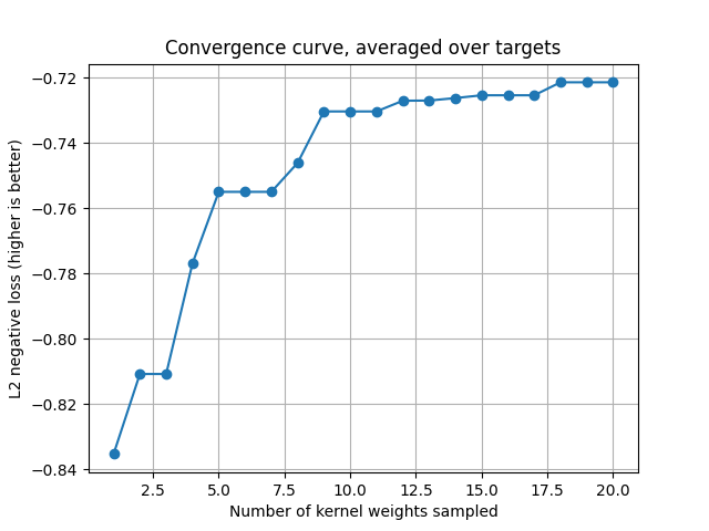
For the random search, cv_scores gives the scores for each sampled kernel
weights vector. The convergence curve is thus the current maximum for each
target.
cv_scores = backend.to_numpy(pipe_1[1].cv_scores_)
current_max = np.maximum.accumulate(cv_scores, axis=0)
mean_current_max = np.mean(current_max, axis=1)

x_array = np.arange(1, len(mean_current_max) + 1)
plt.plot(x_array, mean_current_max, '-o')
plt.grid("on")
plt.xlabel("Number of kernel weights sampled")
plt.ylabel("L2 negative loss (higher is better)")
plt.title("Convergence curve, averaged over targets")
plt.show()

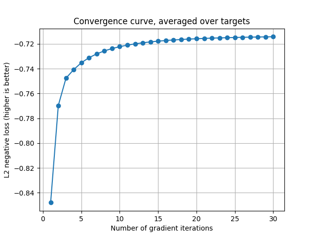
Plot the second convergence curve.
cv_scores = backend.to_numpy(pipe_2[1].cv_scores_)
mean_cv_scores = np.mean(cv_scores, axis=1)

x_array = np.arange(1, len(mean_cv_scores) + 1)
plt.plot(x_array, mean_cv_scores, '-o')
plt.grid("on")
plt.xlabel("Number of gradient iterations")
plt.ylabel("L2 negative loss (higher is better)")
plt.title("Convergence curve, averaged over targets")
plt.show()

Compare with a KernelRidgeCV
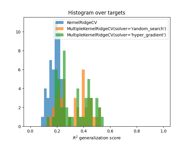
Compare to a baseline KernelRidgeCV model with all the concatenated
features. Comparison is performed using the prediction scores on the test
set.
# Fit the baseline model ``KernelRidgeCV``
baseline = KernelRidgeCV(kernel="linear", alphas=alphas)
baseline.fit(X_train, Y_train)
Compute scores of all models
scores_1 = pipe_1.score(X_test, Y_test)
scores_1 = backend.to_numpy(scores_1)

scores_2 = pipe_2.score(X_test, Y_test)
scores_2 = backend.to_numpy(scores_2)

scores_baseline = baseline.score(X_test, Y_test)
scores_baseline = backend.to_numpy(scores_baseline)
Plot histograms
bins = np.linspace(0, 1, 50)
plt.hist(scores_baseline, bins, alpha=0.7, label="KernelRidgeCV")
plt.hist(scores_1, bins, alpha=0.7,
         label="MultipleKernelRidgeCV(solver='random_search')")
plt.hist(scores_2, bins, alpha=0.7,
         label="MultipleKernelRidgeCV(solver='hyper_gradient')")
plt.xlabel(r"$R^2$ generalization score")
plt.title("Histogram over targets")
plt.legend()
plt.show()

Generate trajectories
Refit the second model with different number of iterations, just to plot the trajectories.
all_kernel_weights_2 = [
    np.full((n_targets, n_kernels), fill_value=1. / n_kernels),
]
max_iter = model_2.solver_params["max_iter"]
for n_iter in np.unique(np.int_(np.logspace(0, np.log10(max_iter), 3))):
    # change the number of iteration and refit from scratch
    pipe_2[1].solver_params['max_iter'] = n_iter
    pipe_2.fit(X_train, Y_train)

    kernel_weights_2 = np.exp(backend.to_numpy(pipe_2[1].deltas_.T))
    kernel_weights_2 /= kernel_weights_2.sum(1)[:, None]
    all_kernel_weights_2.append(kernel_weights_2)
[                              ] 0% | 0.00 sec | hypergradient_direct |
[                              ] 0% | 0.00 sec | hypergradient_direct |
[..............................] 100% | 3.03 sec | hypergradient_direct | 0.33 it/s, ETA: 00:00:00

[                              ] 0% | 0.00 sec | hypergradient_direct |
[                              ] 0% | 0.00 sec | hypergradient_direct |
[......                        ] 20% | 2.96 sec | hypergradient_direct | 0.34 it/s, ETA: 00:00:11
[............                  ] 40% | 3.21 sec | hypergradient_direct | 0.62 it/s, ETA: 00:00:04
[..................            ] 60% | 3.44 sec | hypergradient_direct | 0.87 it/s, ETA: 00:00:02
[........................      ] 80% | 3.69 sec | hypergradient_direct | 1.08 it/s, ETA: 00:00:00
[..............................] 100% | 3.98 sec | hypergradient_direct | 1.26 it/s, ETA: 00:00:00

[                              ] 0% | 0.00 sec | hypergradient_direct |
[                              ] 0% | 0.00 sec | hypergradient_direct |
[.                             ] 3% | 2.96 sec | hypergradient_direct | 0.34 it/s, ETA: 00:01:22
[..                            ] 7% | 3.21 sec | hypergradient_direct | 0.62 it/s, ETA: 00:00:43
[...                           ] 10% | 3.46 sec | hypergradient_direct | 0.87 it/s, ETA: 00:00:29
[....                          ] 14% | 3.70 sec | hypergradient_direct | 1.08 it/s, ETA: 00:00:23
[.....                         ] 17% | 3.95 sec | hypergradient_direct | 1.27 it/s, ETA: 00:00:18
[......                        ] 21% | 4.20 sec | hypergradient_direct | 1.43 it/s, ETA: 00:00:16
[.......                       ] 24% | 4.44 sec | hypergradient_direct | 1.58 it/s, ETA: 00:00:13
[........                      ] 28% | 4.69 sec | hypergradient_direct | 1.71 it/s, ETA: 00:00:12
[.........                     ] 31% | 4.94 sec | hypergradient_direct | 1.82 it/s, ETA: 00:00:10
[..........                    ] 34% | 5.19 sec | hypergradient_direct | 1.93 it/s, ETA: 00:00:09
[...........                   ] 38% | 5.44 sec | hypergradient_direct | 2.02 it/s, ETA: 00:00:08
[............                  ] 41% | 5.69 sec | hypergradient_direct | 2.11 it/s, ETA: 00:00:08
[.............                 ] 45% | 5.93 sec | hypergradient_direct | 2.19 it/s, ETA: 00:00:07
[..............                ] 48% | 6.17 sec | hypergradient_direct | 2.27 it/s, ETA: 00:00:06
[...............               ] 52% | 6.42 sec | hypergradient_direct | 2.34 it/s, ETA: 00:00:05
[................              ] 55% | 6.66 sec | hypergradient_direct | 2.40 it/s, ETA: 00:00:05
[.................             ] 59% | 6.91 sec | hypergradient_direct | 2.46 it/s, ETA: 00:00:04
[..................            ] 62% | 7.15 sec | hypergradient_direct | 2.52 it/s, ETA: 00:00:04
[...................           ] 66% | 7.40 sec | hypergradient_direct | 2.57 it/s, ETA: 00:00:03
[....................          ] 69% | 7.64 sec | hypergradient_direct | 2.62 it/s, ETA: 00:00:03
[.....................         ] 72% | 7.88 sec | hypergradient_direct | 2.67 it/s, ETA: 00:00:03
[......................        ] 76% | 8.12 sec | hypergradient_direct | 2.71 it/s, ETA: 00:00:02
[.......................       ] 79% | 8.37 sec | hypergradient_direct | 2.75 it/s, ETA: 00:00:02
[........................      ] 83% | 8.61 sec | hypergradient_direct | 2.79 it/s, ETA: 00:00:01
[.........................     ] 86% | 8.86 sec | hypergradient_direct | 2.82 it/s, ETA: 00:00:01
[..........................    ] 90% | 9.10 sec | hypergradient_direct | 2.86 it/s, ETA: 00:00:01
[...........................   ] 93% | 9.35 sec | hypergradient_direct | 2.89 it/s, ETA: 00:00:00
[............................  ] 97% | 9.59 sec | hypergradient_direct | 2.92 it/s, ETA: 00:00:00
[..............................] 100% | 9.90 sec | hypergradient_direct | 2.93 it/s, ETA: 00:00:00
Get the normalized kernel weights for the first model
kernel_weights_1 = np.exp(backend.to_numpy(pipe_1[1].deltas_.T))
kernel_weights_1 /= kernel_weights_1.sum(1)[:, None]
Plot on the simplex
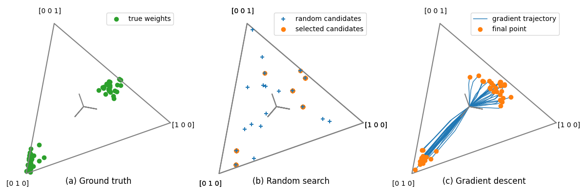
Finally, we visualize the obtained kernel weights vector, projected on the simplex. The simplex is the space of positive weights that sum to one, and it has a triangular shape in dimension 3.
We plot on three different panels:
the kernel weights used in the simulated data
the kernel weights sampled during random search, and the best ones
the kernel weights trajectories obtained during hyper-gradient descent
def _create_simplex_projection_and_edges(ax):
    """Create a projection on the 3D simplex, and plot edges."""
    n_kernels = 3

    if ax is None:
        ax = plt.gca()

    # create a projection in 2D
    from sklearn.decomposition import PCA
    kernel_weights = generate_dirichlet_samples(10000, n_kernels,
                                                concentration=[1.],
                                                random_state=0)
    pca = PCA(2).fit(backend.to_numpy(kernel_weights))

    # add simplex edges
    edges = np.array([[1, 0, 0], [0, 1, 0], [0, 0, 1], [1, 0, 0]])
    edges = pca.transform(edges).T

    # add tripod at origin
    tripod_length = 0.15
    tripod = np.array([[0, 0, 0], [tripod_length, 0, 0], [0, 0, 0],
                       [0, tripod_length, 0], [0, 0, 0], [0, 0,
                                                          tripod_length]])
    tripod = pca.transform(tripod).T

    # add point legend
    points = np.array([[1, 0, 0], [0, 1, 0], [0, 0, 1]])
    labels = points.copy()
    points = pca.transform(points * 1.15).T
    for (xx, yy), label in zip(points.T, labels):
        ax.text(xx, yy, str(label), horizontalalignment='center',
                verticalalignment='center')

    if ax is None:
        plt.figure(figsize=(8, 8))
        ax = plt.gca()
    ax.plot(edges[0], edges[1], c='gray')
    ax.plot(tripod[0], tripod[1], c='gray')
    ax.axis('equal')
    ax.axis('off')
    return ax, pca


def plot_simplex(X, ax=None, **kwargs):
    """Plot a set of points in the 3D simplex."""
    ax, pca = _create_simplex_projection_and_edges(ax=ax)

    Xt = pca.transform(X).T
    ax.scatter(Xt[0], Xt[1], **kwargs)
    ax.legend()
    return ax


def plot_simplex_trajectory(Xs, ax=None):
    """Plot a series of trajectory in the 3D simplex."""
    ax, pca = _create_simplex_projection_and_edges(ax=ax)

    trajectories = []
    for Xi in Xs:
        Xt = pca.transform(Xi).T
        trajectories.append(Xt)
    trajectories = np.array(trajectories)

    for trajectory in trajectories.T:
        ax.plot(trajectory[0], trajectory[1], linewidth=1, color="C0",
                zorder=1)
        ax.scatter(trajectory[0, -1], trajectory[1, -1], color="C1", zorder=2)

    return ax
fig, axs = plt.subplots(1, 3, figsize=(12, 4))

# selection of targets
selection = slice(0, 50)

# First panel
ax = axs[0]
ax.set_title("(a) Ground truth", y=0)
plot_simplex(kernel_weights[selection], ax=ax, color='C2',
             label="true weights")

# Second panel
ax = axs[1]
ax.set_title("(b) Random search", y=0)
plot_simplex(backend.to_numpy(kernel_weights_sampled), ax=ax, marker='+',
             label="random candidates", zorder=10)
plot_simplex(kernel_weights_1[selection], ax=axs[1],
             label="selected candidates")

# Third panel
ax = axs[2]
ax.set_title("(c) Gradient descent", y=0)
plot_simplex_trajectory([aa[selection] for aa in all_kernel_weights_2], ax=ax)
ax.legend([ax.lines[2], ax.collections[0]],
          ['gradient trajectory', 'final point'])

plt.tight_layout()
# fig.savefig('simulation.pdf', dpi=150, bbox_inches='tight', pad_inches=0)
plt.show()

Total running time of the script: (1 minutes 7.068 seconds)