Note
Go to the end to download the full example code.
Multiple-kernel ridge with scikit-learn API
This example demonstrates how to solve multiple kernel ridge regression, using scikit-learn API.
import numpy as np
import matplotlib.pyplot as plt

from himalaya.backend import set_backend
from himalaya.kernel_ridge import KernelRidgeCV
from himalaya.kernel_ridge import MultipleKernelRidgeCV
from himalaya.kernel_ridge import Kernelizer
from himalaya.kernel_ridge import ColumnKernelizer
from himalaya.utils import generate_multikernel_dataset

from sklearn.pipeline import make_pipeline
from sklearn import set_config
set_config(display='diagram')
In this example, we use the torch_cuda backend.
Torch can perform computations both on CPU and GPU. To use CPU, use the “torch” backend, to use GPU, use the “torch_cuda” backend.
backend = set_backend("torch_cuda", on_error="warn")
/home/runner/work/himalaya/himalaya/himalaya/backend/_utils.py:66: UserWarning: Setting backend to torch_cuda failed: PyTorch with CUDA is not available..Falling back to numpy backend.
  warnings.warn(f"Setting backend to {backend} failed: {str(error)}."
Generate a random dataset
X_train : array of shape (n_samples_train, n_features)
X_test : array of shape (n_samples_test, n_features)
Y_train : array of shape (n_samples_train, n_targets)
Y_test : array of shape (n_samples_test, n_targets)
(X_train, X_test, Y_train, Y_test, kernel_weights,
 n_features_list) = generate_multikernel_dataset(n_kernels=3, n_targets=50,
                                                 n_samples_train=600,
                                                 n_samples_test=300,
                                                 random_state=42)

feature_names = [f"Feature space {ii}" for ii in range(len(n_features_list))]
We could precompute the kernels by hand on Xs_train, as done in
plot_mkr_random_search.py. Instead, here we use the ColumnKernelizer
to make a scikit-learn Pipeline.
# Find the start and end of each feature space X in Xs
start_and_end = np.concatenate([[0], np.cumsum(n_features_list)])
slices = [
    slice(start, end)
    for start, end in zip(start_and_end[:-1], start_and_end[1:])
]
Create a different Kernelizer for each feature space. Here we use a
linear kernel for all feature spaces, but ColumnKernelizer accepts any
Kernelizer, or scikit-learn Pipeline ending with a
Kernelizer.
kernelizers = [(name, Kernelizer(), slice_)
               for name, slice_ in zip(feature_names, slices)]
column_kernelizer = ColumnKernelizer(kernelizers)

# Note that ``ColumnKernelizer`` has a parameter ``n_jobs`` to parallelize each
# kernelizer, yet such parallelism does not work with GPU arrays.
Define the model
The class takes a number of common parameters during initialization, such as kernels or solver. Since the solver parameters might be different depending on the solver, they can be passed in the solver_params parameter.
Here we use the “random_search” solver. We can check its specific parameters in the function docstring:
solver_function = MultipleKernelRidgeCV.ALL_SOLVERS["random_search"]
print("Docstring of the function %s:" % solver_function.__name__)
print(solver_function.__doc__)
Docstring of the function solve_multiple_kernel_ridge_random_search:
Solve multiple kernel ridge regression using random search.

    Parameters
    ----------
    Ks : array of shape (n_kernels, n_samples, n_samples)
        Input kernels.
    Y : array of shape (n_samples, n_targets)
        Target data.
    n_iter : int, or array of shape (n_iter, n_kernels)
        Number of kernel weights combination to search.
        If an array is given, the solver uses it as the list of kernel weights
        to try, instead of sampling from a Dirichlet distribution. Examples:
          - `n_iter=np.eye(n_kernels)` implement a winner-take-all strategy
            over kernels.
          - `n_iter=np.ones((1, n_kernels))/n_kernels` solves a (standard)
            kernel ridge regression.
    concentration : float, or list of float
        Concentration parameters of the Dirichlet distribution.
        If a list, iteratively cycle through the list.
        Not used if n_iter is an array.
    alphas : float or array of shape (n_alphas, )
        Range of ridge regularization parameter.
    score_func : callable
        Function used to compute the score of predictions versus Y.
    cv : int or scikit-learn splitter
        Cross-validation splitter. If an int, KFold is used.
    fit_intercept : boolean
        Whether to fit an intercept. If False, Ks should be centered
        (see KernelCenterer), and Y must be zero-mean over samples.
        Only available if return_weights == 'dual'.
    return_weights : None, 'primal', or 'dual'
        Whether to refit on the entire dataset and return the weights.
    Xs : array of shape (n_kernels, n_samples, n_features) or None
        Necessary if return_weights == 'primal'.
    local_alpha : bool
        If True, alphas are selected per target, else shared over all targets.
    jitter_alphas : bool
        If True, alphas range is slightly jittered for each gamma.
    random_state : int, or None
        Random generator seed. Use an int for deterministic search.
    n_targets_batch : int or None
        Size of the batch for over targets during cross-validation.
        Used for memory reasons. If None, uses all n_targets at once.
    n_targets_batch_refit : int or None
        Size of the batch for over targets during refit.
        Used for memory reasons. If None, uses all n_targets at once.
    n_alphas_batch : int or None
        Size of the batch for over alphas. Used for memory reasons.
        If None, uses all n_alphas at once.
    progress_bar : bool
        If True, display a progress bar over gammas.
    Ks_in_cpu : bool
        If True, keep Ks in CPU memory to limit GPU memory (slower).
        This feature is not available through the scikit-learn API.
    conservative : bool
        If True, when selecting the hyperparameter alpha, take the largest one
        that is less than one standard deviation away from the best.
        If False, take the best.
    Y_in_cpu : bool
        If True, keep the target values ``Y`` in CPU memory (slower).
    diagonalize_method : str in {"eigh", "svd"}
        Method used to diagonalize the kernel.
    return_alphas : bool
        If True, return the best alpha value for each target.

    Returns
    -------
    deltas : array of shape (n_kernels, n_targets)
        Best log kernel weights for each target.
    refit_weights : array or None
        Refit regression weights on the entire dataset, using selected best
        hyperparameters. Refit weights are always stored on CPU memory.
        If return_weights == 'primal', shape is (n_features, n_targets),
        if return_weights == 'dual', shape is (n_samples, n_targets),
        else, None.
    cv_scores : array of shape (n_iter, n_targets)
        Cross-validation scores per iteration, averaged over splits, for the
        best alpha. Cross-validation scores will always be on CPU memory.
    best_alphas : array of shape (n_targets, )
        Best alpha value per target. Only returned if return_alphas is True.
    intercept : array of shape (n_targets,)
        Intercept. Only returned when fit_intercept is True.
We use 100 iterations to have a reasonably fast example (~40 sec). To have a better convergence, we probably need more iterations. Note that there is currently no stopping criterion in this method.
n_iter = 100
Grid of regularization parameters.
alphas = np.logspace(-10, 10, 41)
Batch parameters are used to reduce the necessary GPU memory. A larger value will be a bit faster, but the solver might crash if it runs out of memory. Optimal values depend on the size of your dataset.
n_targets_batch = 1000
n_alphas_batch = 20
n_targets_batch_refit = 200

solver_params = dict(n_iter=n_iter, alphas=alphas,
                     n_targets_batch=n_targets_batch,
                     n_alphas_batch=n_alphas_batch,
                     n_targets_batch_refit=n_targets_batch_refit,
                     jitter_alphas=True)

model = MultipleKernelRidgeCV(kernels="precomputed", solver="random_search",
                              solver_params=solver_params)
Define and fit the pipeline
pipe = make_pipeline(column_kernelizer, model)
pipe.fit(X_train, Y_train)
[                              ] 0% | 0.00 sec | 100 random sampling with cv |
[                              ] 1% | 1.63 sec | 100 random sampling with cv | 0.61 it/s, ETA: 00:02:41
[                              ] 2% | 2.97 sec | 100 random sampling with cv | 0.67 it/s, ETA: 00:02:25
[                              ] 3% | 4.30 sec | 100 random sampling with cv | 0.70 it/s, ETA: 00:02:19
[.                             ] 4% | 5.62 sec | 100 random sampling with cv | 0.71 it/s, ETA: 00:02:14
[.                             ] 5% | 6.90 sec | 100 random sampling with cv | 0.72 it/s, ETA: 00:02:11
[.                             ] 6% | 8.18 sec | 100 random sampling with cv | 0.73 it/s, ETA: 00:02:08
[..                            ] 7% | 9.36 sec | 100 random sampling with cv | 0.75 it/s, ETA: 00:02:04
[..                            ] 8% | 10.53 sec | 100 random sampling with cv | 0.76 it/s, ETA: 00:02:01
[..                            ] 9% | 11.85 sec | 100 random sampling with cv | 0.76 it/s, ETA: 00:01:59
[...                           ] 10% | 13.04 sec | 100 random sampling with cv | 0.77 it/s, ETA: 00:01:57
[...                           ] 11% | 14.25 sec | 100 random sampling with cv | 0.77 it/s, ETA: 00:01:55
[...                           ] 12% | 15.60 sec | 100 random sampling with cv | 0.77 it/s, ETA: 00:01:54
[...                           ] 13% | 16.73 sec | 100 random sampling with cv | 0.78 it/s, ETA: 00:01:51
[....                          ] 14% | 18.19 sec | 100 random sampling with cv | 0.77 it/s, ETA: 00:01:51
[....                          ] 15% | 19.60 sec | 100 random sampling with cv | 0.77 it/s, ETA: 00:01:51
[....                          ] 16% | 20.73 sec | 100 random sampling with cv | 0.77 it/s, ETA: 00:01:48
[.....                         ] 17% | 22.11 sec | 100 random sampling with cv | 0.77 it/s, ETA: 00:01:47
[.....                         ] 18% | 23.49 sec | 100 random sampling with cv | 0.77 it/s, ETA: 00:01:47
[.....                         ] 19% | 24.63 sec | 100 random sampling with cv | 0.77 it/s, ETA: 00:01:45
[......                        ] 20% | 25.93 sec | 100 random sampling with cv | 0.77 it/s, ETA: 00:01:43
[......                        ] 21% | 27.08 sec | 100 random sampling with cv | 0.78 it/s, ETA: 00:01:41
[......                        ] 22% | 28.43 sec | 100 random sampling with cv | 0.77 it/s, ETA: 00:01:40
[......                        ] 23% | 29.77 sec | 100 random sampling with cv | 0.77 it/s, ETA: 00:01:39
[.......                       ] 24% | 31.03 sec | 100 random sampling with cv | 0.77 it/s, ETA: 00:01:38
[.......                       ] 25% | 32.10 sec | 100 random sampling with cv | 0.78 it/s, ETA: 00:01:36
[.......                       ] 26% | 33.52 sec | 100 random sampling with cv | 0.78 it/s, ETA: 00:01:35
[........                      ] 27% | 34.95 sec | 100 random sampling with cv | 0.77 it/s, ETA: 00:01:34
[........                      ] 28% | 36.14 sec | 100 random sampling with cv | 0.77 it/s, ETA: 00:01:32
[........                      ] 29% | 37.17 sec | 100 random sampling with cv | 0.78 it/s, ETA: 00:01:30
[.........                     ] 30% | 38.17 sec | 100 random sampling with cv | 0.79 it/s, ETA: 00:01:29
[.........                     ] 31% | 39.54 sec | 100 random sampling with cv | 0.78 it/s, ETA: 00:01:28
[.........                     ] 32% | 40.68 sec | 100 random sampling with cv | 0.79 it/s, ETA: 00:01:26
[.........                     ] 33% | 42.02 sec | 100 random sampling with cv | 0.79 it/s, ETA: 00:01:25
[..........                    ] 34% | 43.20 sec | 100 random sampling with cv | 0.79 it/s, ETA: 00:01:23
[..........                    ] 35% | 44.30 sec | 100 random sampling with cv | 0.79 it/s, ETA: 00:01:22
[..........                    ] 36% | 45.44 sec | 100 random sampling with cv | 0.79 it/s, ETA: 00:01:20
[...........                   ] 37% | 46.74 sec | 100 random sampling with cv | 0.79 it/s, ETA: 00:01:19
[...........                   ] 38% | 47.75 sec | 100 random sampling with cv | 0.80 it/s, ETA: 00:01:17
[...........                   ] 39% | 48.91 sec | 100 random sampling with cv | 0.80 it/s, ETA: 00:01:16
[............                  ] 40% | 50.08 sec | 100 random sampling with cv | 0.80 it/s, ETA: 00:01:15
[............                  ] 41% | 51.48 sec | 100 random sampling with cv | 0.80 it/s, ETA: 00:01:14
[............                  ] 42% | 52.63 sec | 100 random sampling with cv | 0.80 it/s, ETA: 00:01:12
[............                  ] 43% | 53.64 sec | 100 random sampling with cv | 0.80 it/s, ETA: 00:01:11
[.............                 ] 44% | 54.71 sec | 100 random sampling with cv | 0.80 it/s, ETA: 00:01:09
[.............                 ] 45% | 55.69 sec | 100 random sampling with cv | 0.81 it/s, ETA: 00:01:08
[.............                 ] 46% | 56.80 sec | 100 random sampling with cv | 0.81 it/s, ETA: 00:01:06
[..............                ] 47% | 58.11 sec | 100 random sampling with cv | 0.81 it/s, ETA: 00:01:05
[..............                ] 48% | 59.33 sec | 100 random sampling with cv | 0.81 it/s, ETA: 00:01:04
[..............                ] 49% | 60.67 sec | 100 random sampling with cv | 0.81 it/s, ETA: 00:01:03
[...............               ] 50% | 61.57 sec | 100 random sampling with cv | 0.81 it/s, ETA: 00:01:01
[...............               ] 51% | 63.00 sec | 100 random sampling with cv | 0.81 it/s, ETA: 00:01:00
[...............               ] 52% | 64.49 sec | 100 random sampling with cv | 0.81 it/s, ETA: 00:00:59
[...............               ] 53% | 65.62 sec | 100 random sampling with cv | 0.81 it/s, ETA: 00:00:58
[................              ] 54% | 67.01 sec | 100 random sampling with cv | 0.81 it/s, ETA: 00:00:57
[................              ] 55% | 68.16 sec | 100 random sampling with cv | 0.81 it/s, ETA: 00:00:55
[................              ] 56% | 69.42 sec | 100 random sampling with cv | 0.81 it/s, ETA: 00:00:54
[.................             ] 57% | 70.50 sec | 100 random sampling with cv | 0.81 it/s, ETA: 00:00:53
[.................             ] 58% | 71.69 sec | 100 random sampling with cv | 0.81 it/s, ETA: 00:00:51
[.................             ] 59% | 72.75 sec | 100 random sampling with cv | 0.81 it/s, ETA: 00:00:50
[..................            ] 60% | 73.74 sec | 100 random sampling with cv | 0.81 it/s, ETA: 00:00:49
[..................            ] 61% | 75.00 sec | 100 random sampling with cv | 0.81 it/s, ETA: 00:00:47
[..................            ] 62% | 76.14 sec | 100 random sampling with cv | 0.81 it/s, ETA: 00:00:46
[..................            ] 63% | 77.39 sec | 100 random sampling with cv | 0.81 it/s, ETA: 00:00:45
[...................           ] 64% | 78.53 sec | 100 random sampling with cv | 0.81 it/s, ETA: 00:00:44
[...................           ] 65% | 79.66 sec | 100 random sampling with cv | 0.82 it/s, ETA: 00:00:42
[...................           ] 66% | 80.85 sec | 100 random sampling with cv | 0.82 it/s, ETA: 00:00:41
[....................          ] 67% | 82.26 sec | 100 random sampling with cv | 0.81 it/s, ETA: 00:00:40
[....................          ] 68% | 83.44 sec | 100 random sampling with cv | 0.81 it/s, ETA: 00:00:39
[....................          ] 69% | 84.57 sec | 100 random sampling with cv | 0.82 it/s, ETA: 00:00:37
[.....................         ] 70% | 85.91 sec | 100 random sampling with cv | 0.81 it/s, ETA: 00:00:36
[.....................         ] 71% | 87.16 sec | 100 random sampling with cv | 0.81 it/s, ETA: 00:00:35
[.....................         ] 72% | 88.46 sec | 100 random sampling with cv | 0.81 it/s, ETA: 00:00:34
[.....................         ] 73% | 89.47 sec | 100 random sampling with cv | 0.82 it/s, ETA: 00:00:33
[......................        ] 74% | 90.49 sec | 100 random sampling with cv | 0.82 it/s, ETA: 00:00:31
[......................        ] 75% | 91.77 sec | 100 random sampling with cv | 0.82 it/s, ETA: 00:00:30
[......................        ] 76% | 93.17 sec | 100 random sampling with cv | 0.82 it/s, ETA: 00:00:29
[.......................       ] 77% | 94.20 sec | 100 random sampling with cv | 0.82 it/s, ETA: 00:00:28
[.......................       ] 78% | 95.16 sec | 100 random sampling with cv | 0.82 it/s, ETA: 00:00:26
[.......................       ] 79% | 96.35 sec | 100 random sampling with cv | 0.82 it/s, ETA: 00:00:25
[........................      ] 80% | 97.63 sec | 100 random sampling with cv | 0.82 it/s, ETA: 00:00:24
[........................      ] 81% | 98.71 sec | 100 random sampling with cv | 0.82 it/s, ETA: 00:00:23
[........................      ] 82% | 99.88 sec | 100 random sampling with cv | 0.82 it/s, ETA: 00:00:21
[........................      ] 83% | 100.91 sec | 100 random sampling with cv | 0.82 it/s, ETA: 00:00:20
[.........................     ] 84% | 102.12 sec | 100 random sampling with cv | 0.82 it/s, ETA: 00:00:19
[.........................     ] 85% | 103.31 sec | 100 random sampling with cv | 0.82 it/s, ETA: 00:00:18
[.........................     ] 86% | 104.45 sec | 100 random sampling with cv | 0.82 it/s, ETA: 00:00:17
[..........................    ] 87% | 105.72 sec | 100 random sampling with cv | 0.82 it/s, ETA: 00:00:15
[..........................    ] 88% | 107.13 sec | 100 random sampling with cv | 0.82 it/s, ETA: 00:00:14
[..........................    ] 89% | 108.24 sec | 100 random sampling with cv | 0.82 it/s, ETA: 00:00:13
[...........................   ] 90% | 109.44 sec | 100 random sampling with cv | 0.82 it/s, ETA: 00:00:12
[...........................   ] 91% | 110.56 sec | 100 random sampling with cv | 0.82 it/s, ETA: 00:00:10
[...........................   ] 92% | 111.74 sec | 100 random sampling with cv | 0.82 it/s, ETA: 00:00:09
[...........................   ] 93% | 113.04 sec | 100 random sampling with cv | 0.82 it/s, ETA: 00:00:08
[............................  ] 94% | 114.39 sec | 100 random sampling with cv | 0.82 it/s, ETA: 00:00:07
[............................  ] 95% | 115.62 sec | 100 random sampling with cv | 0.82 it/s, ETA: 00:00:06
[............................  ] 96% | 116.89 sec | 100 random sampling with cv | 0.82 it/s, ETA: 00:00:04
[............................. ] 97% | 118.10 sec | 100 random sampling with cv | 0.82 it/s, ETA: 00:00:03
[............................. ] 98% | 119.49 sec | 100 random sampling with cv | 0.82 it/s, ETA: 00:00:02
[............................. ] 99% | 121.07 sec | 100 random sampling with cv | 0.82 it/s, ETA: 00:00:01
[..............................] 100% | 122.16 sec | 100 random sampling with cv | 0.82 it/s, ETA: 00:00:00
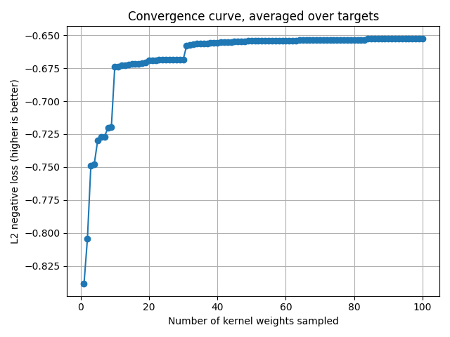
Plot the convergence curve
# ``cv_scores`` gives the scores for each sampled kernel weights.
# The convergence curve is thus the current maximum for each target.
cv_scores = backend.to_numpy(pipe[1].cv_scores_)
current_max = np.maximum.accumulate(cv_scores, axis=0)
mean_current_max = np.mean(current_max, axis=1)

x_array = np.arange(1, len(mean_current_max) + 1)
plt.plot(x_array, mean_current_max, '-o')
plt.grid("on")
plt.xlabel("Number of kernel weights sampled")
plt.ylabel("L2 negative loss (higher is better)")
plt.title("Convergence curve, averaged over targets")
plt.tight_layout()
plt.show()
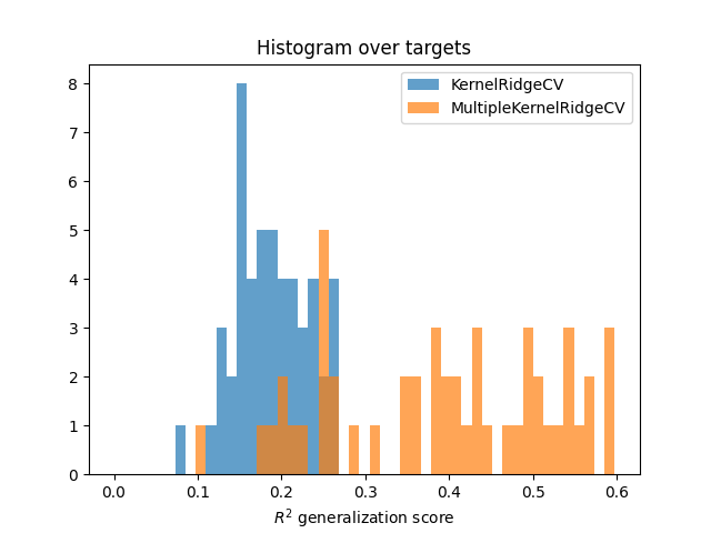
Compare to KernelRidgeCV
Compare to a baseline KernelRidgeCV model with all the concatenated
features. Comparison is performed using the prediction scores on the test
set.
Fit the baseline model KernelRidgeCV
baseline = KernelRidgeCV(kernel="linear", alphas=alphas)
baseline.fit(X_train, Y_train)
Compute scores of both models
scores = pipe.score(X_test, Y_test)
scores = backend.to_numpy(scores)

scores_baseline = baseline.score(X_test, Y_test)
scores_baseline = backend.to_numpy(scores_baseline)
Plot histograms
bins = np.linspace(0, max(scores_baseline.max(), scores.max()), 50)
plt.hist(scores_baseline, bins, alpha=0.7, label="KernelRidgeCV")
plt.hist(scores, bins, alpha=0.7, label="MultipleKernelRidgeCV")
plt.xlabel(r"$R^2$ generalization score")
plt.title("Histogram over targets")
plt.legend()
plt.show()
Total running time of the script: (2 minutes 5.183 seconds)