Note
Go to the end to download the full example code.
Multiple-kernel ridge
This example demonstrates how to solve multiple kernel ridge regression. It uses random search and cross validation to select optimal hyperparameters.
import numpy as np
import matplotlib.pyplot as plt

from himalaya.backend import set_backend
from himalaya.kernel_ridge import solve_multiple_kernel_ridge_random_search
from himalaya.kernel_ridge import predict_and_score_weighted_kernel_ridge
from himalaya.utils import generate_multikernel_dataset
from himalaya.scoring import r2_score_split
from himalaya.viz import plot_alphas_diagnostic
In this example, we use the cupy backend, and fit the model on GPU.
backend = set_backend("cupy", on_error="warn")
/home/runner/work/himalaya/himalaya/himalaya/backend/_utils.py:66: UserWarning: Setting backend to cupy failed: Cupy not installed..Falling back to numpy backend.
  warnings.warn(f"Setting backend to {backend} failed: {str(error)}."
Generate a random dataset
X_train : array of shape (n_samples_train, n_features)
X_test : array of shape (n_samples_test, n_features)
Y_train : array of shape (n_samples_train, n_targets)
Y_test : array of shape (n_samples_test, n_targets)
n_kernels = 3
n_targets = 50
kernel_weights = np.tile(np.array([0.5, 0.3, 0.2])[None], (n_targets, 1))

(X_train, X_test, Y_train, Y_test,
 kernel_weights, n_features_list) = generate_multikernel_dataset(
     n_kernels=n_kernels, n_targets=n_targets, n_samples_train=600,
     n_samples_test=300, kernel_weights=kernel_weights, random_state=42)

feature_names = [f"Feature space {ii}" for ii in range(len(n_features_list))]

# Find the start and end of each feature space X in Xs
start_and_end = np.concatenate([[0], np.cumsum(n_features_list)])
slices = [
    slice(start, end)
    for start, end in zip(start_and_end[:-1], start_and_end[1:])
]
Xs_train = [X_train[:, slic] for slic in slices]
Xs_test = [X_test[:, slic] for slic in slices]
Precompute the linear kernels
We also cast them to float32.
Ks_train = backend.stack([X_train @ X_train.T for X_train in Xs_train])
Ks_train = backend.asarray(Ks_train, dtype=backend.float32)
Y_train = backend.asarray(Y_train, dtype=backend.float32)

Ks_test = backend.stack(
    [X_test @ X_train.T for X_train, X_test in zip(Xs_train, Xs_test)])
Ks_test = backend.asarray(Ks_test, dtype=backend.float32)
Y_test = backend.asarray(Y_test, dtype=backend.float32)
Run the solver, using random search
This method should work fine for
small number of kernels (< 20). The larger the number of kernels, the larger
we need to sample the hyperparameter space (i.e. increasing n_iter).
Here we use 100 iterations to have a reasonably fast example (~40 sec). To have a better convergence, we probably need more iterations. Note that there is currently no stopping criterion in this method.
n_iter = 100
Grid of regularization parameters.
alphas = np.logspace(-10, 10, 21)
Batch parameters are used to reduce the necessary GPU memory. A larger value will be a bit faster, but the solver might crash if it runs out of memory. Optimal values depend on the size of your dataset.
n_targets_batch = 1000
n_alphas_batch = 20
If return_weights == "dual", the solver will use more memory.
To mitigate this, you can reduce n_targets_batch in the refit
using `n_targets_batch_refit.
If you don’t need the dual weights, use return_weights = None.
return_weights = 'dual'
n_targets_batch_refit = 200
Run the solver. For each iteration, it will:
sample kernel weights from a Dirichlet distribution
fit (n_splits * n_alphas * n_targets) ridge models
compute the scores on the validation set of each split
average the scores over splits
take the maximum over alphas
(only if you ask for the ridge weights) refit using the best alphas per target and the entire dataset
return for each target the log kernel weights leading to the best CV score (and the best weights if necessary)
results = solve_multiple_kernel_ridge_random_search(
    Ks=Ks_train,
    Y=Y_train,
    n_iter=n_iter,
    alphas=alphas,
    n_targets_batch=n_targets_batch,
    return_weights=return_weights,
    n_alphas_batch=n_alphas_batch,
    n_targets_batch_refit=n_targets_batch_refit,
    jitter_alphas=True,
)
[                              ] 0% | 0.00 sec | 100 random sampling with cv |
[                              ] 1% | 1.40 sec | 100 random sampling with cv | 0.72 it/s, ETA: 00:02:18
[                              ] 2% | 2.66 sec | 100 random sampling with cv | 0.75 it/s, ETA: 00:02:10
[                              ] 3% | 3.40 sec | 100 random sampling with cv | 0.88 it/s, ETA: 00:01:49
[.                             ] 4% | 4.32 sec | 100 random sampling with cv | 0.93 it/s, ETA: 00:01:43
[.                             ] 5% | 5.30 sec | 100 random sampling with cv | 0.94 it/s, ETA: 00:01:40
[.                             ] 6% | 6.37 sec | 100 random sampling with cv | 0.94 it/s, ETA: 00:01:39
[..                            ] 7% | 7.43 sec | 100 random sampling with cv | 0.94 it/s, ETA: 00:01:38
[..                            ] 8% | 8.54 sec | 100 random sampling with cv | 0.94 it/s, ETA: 00:01:38
[..                            ] 9% | 9.53 sec | 100 random sampling with cv | 0.94 it/s, ETA: 00:01:36
[...                           ] 10% | 10.62 sec | 100 random sampling with cv | 0.94 it/s, ETA: 00:01:35
[...                           ] 11% | 12.01 sec | 100 random sampling with cv | 0.92 it/s, ETA: 00:01:37
[...                           ] 12% | 13.43 sec | 100 random sampling with cv | 0.89 it/s, ETA: 00:01:38
[...                           ] 13% | 14.21 sec | 100 random sampling with cv | 0.91 it/s, ETA: 00:01:35
[....                          ] 14% | 15.22 sec | 100 random sampling with cv | 0.92 it/s, ETA: 00:01:33
[....                          ] 15% | 16.08 sec | 100 random sampling with cv | 0.93 it/s, ETA: 00:01:31
[....                          ] 16% | 17.17 sec | 100 random sampling with cv | 0.93 it/s, ETA: 00:01:30
[.....                         ] 17% | 18.35 sec | 100 random sampling with cv | 0.93 it/s, ETA: 00:01:29
[.....                         ] 18% | 19.27 sec | 100 random sampling with cv | 0.93 it/s, ETA: 00:01:27
[.....                         ] 19% | 20.09 sec | 100 random sampling with cv | 0.95 it/s, ETA: 00:01:25
[......                        ] 20% | 21.10 sec | 100 random sampling with cv | 0.95 it/s, ETA: 00:01:24
[......                        ] 21% | 22.19 sec | 100 random sampling with cv | 0.95 it/s, ETA: 00:01:23
[......                        ] 22% | 23.18 sec | 100 random sampling with cv | 0.95 it/s, ETA: 00:01:22
[......                        ] 23% | 24.35 sec | 100 random sampling with cv | 0.94 it/s, ETA: 00:01:21
[.......                       ] 24% | 25.28 sec | 100 random sampling with cv | 0.95 it/s, ETA: 00:01:20
[.......                       ] 25% | 26.05 sec | 100 random sampling with cv | 0.96 it/s, ETA: 00:01:18
[.......                       ] 26% | 27.02 sec | 100 random sampling with cv | 0.96 it/s, ETA: 00:01:16
[........                      ] 27% | 27.82 sec | 100 random sampling with cv | 0.97 it/s, ETA: 00:01:15
[........                      ] 28% | 28.85 sec | 100 random sampling with cv | 0.97 it/s, ETA: 00:01:14
[........                      ] 29% | 29.86 sec | 100 random sampling with cv | 0.97 it/s, ETA: 00:01:13
[.........                     ] 30% | 30.64 sec | 100 random sampling with cv | 0.98 it/s, ETA: 00:01:11
[.........                     ] 31% | 31.34 sec | 100 random sampling with cv | 0.99 it/s, ETA: 00:01:09
[.........                     ] 32% | 32.43 sec | 100 random sampling with cv | 0.99 it/s, ETA: 00:01:08
[.........                     ] 33% | 33.40 sec | 100 random sampling with cv | 0.99 it/s, ETA: 00:01:07
[..........                    ] 34% | 34.29 sec | 100 random sampling with cv | 0.99 it/s, ETA: 00:01:06
[..........                    ] 35% | 35.12 sec | 100 random sampling with cv | 1.00 it/s, ETA: 00:01:05
[..........                    ] 36% | 36.05 sec | 100 random sampling with cv | 1.00 it/s, ETA: 00:01:04
[...........                   ] 37% | 36.96 sec | 100 random sampling with cv | 1.00 it/s, ETA: 00:01:02
[...........                   ] 38% | 37.76 sec | 100 random sampling with cv | 1.01 it/s, ETA: 00:01:01
[...........                   ] 39% | 38.78 sec | 100 random sampling with cv | 1.01 it/s, ETA: 00:01:00
[............                  ] 40% | 39.71 sec | 100 random sampling with cv | 1.01 it/s, ETA: 00:00:59
[............                  ] 41% | 40.73 sec | 100 random sampling with cv | 1.01 it/s, ETA: 00:00:58
[............                  ] 42% | 41.64 sec | 100 random sampling with cv | 1.01 it/s, ETA: 00:00:57
[............                  ] 43% | 42.79 sec | 100 random sampling with cv | 1.00 it/s, ETA: 00:00:56
[.............                 ] 44% | 43.81 sec | 100 random sampling with cv | 1.00 it/s, ETA: 00:00:55
[.............                 ] 45% | 44.88 sec | 100 random sampling with cv | 1.00 it/s, ETA: 00:00:54
[.............                 ] 46% | 45.92 sec | 100 random sampling with cv | 1.00 it/s, ETA: 00:00:53
[..............                ] 47% | 47.06 sec | 100 random sampling with cv | 1.00 it/s, ETA: 00:00:53
[..............                ] 48% | 48.22 sec | 100 random sampling with cv | 1.00 it/s, ETA: 00:00:52
[..............                ] 49% | 49.06 sec | 100 random sampling with cv | 1.00 it/s, ETA: 00:00:51
[...............               ] 50% | 49.84 sec | 100 random sampling with cv | 1.00 it/s, ETA: 00:00:49
[...............               ] 51% | 50.52 sec | 100 random sampling with cv | 1.01 it/s, ETA: 00:00:48
[...............               ] 52% | 51.47 sec | 100 random sampling with cv | 1.01 it/s, ETA: 00:00:47
[...............               ] 53% | 52.52 sec | 100 random sampling with cv | 1.01 it/s, ETA: 00:00:46
[................              ] 54% | 53.58 sec | 100 random sampling with cv | 1.01 it/s, ETA: 00:00:45
[................              ] 55% | 54.72 sec | 100 random sampling with cv | 1.01 it/s, ETA: 00:00:44
[................              ] 56% | 55.71 sec | 100 random sampling with cv | 1.01 it/s, ETA: 00:00:43
[.................             ] 57% | 56.66 sec | 100 random sampling with cv | 1.01 it/s, ETA: 00:00:42
[.................             ] 58% | 57.79 sec | 100 random sampling with cv | 1.00 it/s, ETA: 00:00:41
[.................             ] 59% | 58.93 sec | 100 random sampling with cv | 1.00 it/s, ETA: 00:00:40
[..................            ] 60% | 59.77 sec | 100 random sampling with cv | 1.00 it/s, ETA: 00:00:39
[..................            ] 61% | 60.62 sec | 100 random sampling with cv | 1.01 it/s, ETA: 00:00:38
[..................            ] 62% | 61.82 sec | 100 random sampling with cv | 1.00 it/s, ETA: 00:00:37
[..................            ] 63% | 62.39 sec | 100 random sampling with cv | 1.01 it/s, ETA: 00:00:36
[...................           ] 64% | 63.39 sec | 100 random sampling with cv | 1.01 it/s, ETA: 00:00:35
[...................           ] 65% | 64.39 sec | 100 random sampling with cv | 1.01 it/s, ETA: 00:00:34
[...................           ] 66% | 65.31 sec | 100 random sampling with cv | 1.01 it/s, ETA: 00:00:33
[....................          ] 67% | 66.18 sec | 100 random sampling with cv | 1.01 it/s, ETA: 00:00:32
[....................          ] 68% | 66.94 sec | 100 random sampling with cv | 1.02 it/s, ETA: 00:00:31
[....................          ] 69% | 67.70 sec | 100 random sampling with cv | 1.02 it/s, ETA: 00:00:30
[.....................         ] 70% | 68.81 sec | 100 random sampling with cv | 1.02 it/s, ETA: 00:00:29
[.....................         ] 71% | 69.81 sec | 100 random sampling with cv | 1.02 it/s, ETA: 00:00:28
[.....................         ] 72% | 71.08 sec | 100 random sampling with cv | 1.01 it/s, ETA: 00:00:27
[.....................         ] 73% | 71.94 sec | 100 random sampling with cv | 1.01 it/s, ETA: 00:00:26
[......................        ] 74% | 72.78 sec | 100 random sampling with cv | 1.02 it/s, ETA: 00:00:25
[......................        ] 75% | 73.71 sec | 100 random sampling with cv | 1.02 it/s, ETA: 00:00:24
[......................        ] 76% | 74.76 sec | 100 random sampling with cv | 1.02 it/s, ETA: 00:00:23
[.......................       ] 77% | 75.70 sec | 100 random sampling with cv | 1.02 it/s, ETA: 00:00:22
[.......................       ] 78% | 76.79 sec | 100 random sampling with cv | 1.02 it/s, ETA: 00:00:21
[.......................       ] 79% | 77.60 sec | 100 random sampling with cv | 1.02 it/s, ETA: 00:00:20
[........................      ] 80% | 78.55 sec | 100 random sampling with cv | 1.02 it/s, ETA: 00:00:19
[........................      ] 81% | 79.49 sec | 100 random sampling with cv | 1.02 it/s, ETA: 00:00:18
[........................      ] 82% | 80.26 sec | 100 random sampling with cv | 1.02 it/s, ETA: 00:00:17
[........................      ] 83% | 81.37 sec | 100 random sampling with cv | 1.02 it/s, ETA: 00:00:16
[.........................     ] 84% | 82.20 sec | 100 random sampling with cv | 1.02 it/s, ETA: 00:00:15
[.........................     ] 85% | 82.90 sec | 100 random sampling with cv | 1.03 it/s, ETA: 00:00:14
[.........................     ] 86% | 83.75 sec | 100 random sampling with cv | 1.03 it/s, ETA: 00:00:13
[..........................    ] 87% | 84.59 sec | 100 random sampling with cv | 1.03 it/s, ETA: 00:00:12
[..........................    ] 88% | 85.62 sec | 100 random sampling with cv | 1.03 it/s, ETA: 00:00:11
[..........................    ] 89% | 86.41 sec | 100 random sampling with cv | 1.03 it/s, ETA: 00:00:10
[...........................   ] 90% | 87.73 sec | 100 random sampling with cv | 1.03 it/s, ETA: 00:00:09
[...........................   ] 91% | 88.56 sec | 100 random sampling with cv | 1.03 it/s, ETA: 00:00:08
[...........................   ] 92% | 89.45 sec | 100 random sampling with cv | 1.03 it/s, ETA: 00:00:07
[...........................   ] 93% | 90.49 sec | 100 random sampling with cv | 1.03 it/s, ETA: 00:00:06
[............................  ] 94% | 91.51 sec | 100 random sampling with cv | 1.03 it/s, ETA: 00:00:05
[............................  ] 95% | 92.24 sec | 100 random sampling with cv | 1.03 it/s, ETA: 00:00:04
[............................  ] 96% | 93.17 sec | 100 random sampling with cv | 1.03 it/s, ETA: 00:00:03
[............................. ] 97% | 94.11 sec | 100 random sampling with cv | 1.03 it/s, ETA: 00:00:02
[............................. ] 98% | 94.98 sec | 100 random sampling with cv | 1.03 it/s, ETA: 00:00:01
[............................. ] 99% | 95.94 sec | 100 random sampling with cv | 1.03 it/s, ETA: 00:00:00
[..............................] 100% | 96.75 sec | 100 random sampling with cv | 1.03 it/s, ETA: 00:00:00
As we used the cupy backend, the results are cupy arrays, which are
on GPU. Here, we cast the results back to CPU, and to numpy arrays.
deltas = backend.to_numpy(results[0])
dual_weights = backend.to_numpy(results[1])
cv_scores = backend.to_numpy(results[2])
Plot the convergence curve
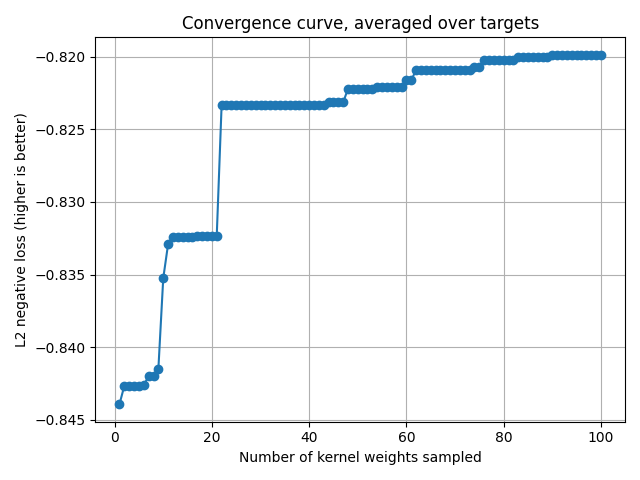
cv_scores gives the scores for each sampled kernel weights.
The convergence curve is thus the current maximum for each target.
current_max = np.maximum.accumulate(cv_scores, axis=0)
mean_current_max = np.mean(current_max, axis=1)
x_array = np.arange(1, len(mean_current_max) + 1)
plt.plot(x_array, mean_current_max, '-o')
plt.grid("on")
plt.xlabel("Number of kernel weights sampled")
plt.ylabel("L2 negative loss (higher is better)")
plt.title("Convergence curve, averaged over targets")
plt.tight_layout()
plt.show()

Plot the optimal alphas selected by the solver
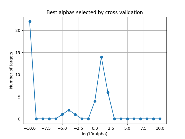
This plot is helpful to refine the alpha grid if the range is too small or too large.
best_alphas = 1. / np.sum(np.exp(deltas), axis=0)
plot_alphas_diagnostic(best_alphas, alphas)
plt.title("Best alphas selected by cross-validation")
plt.show()

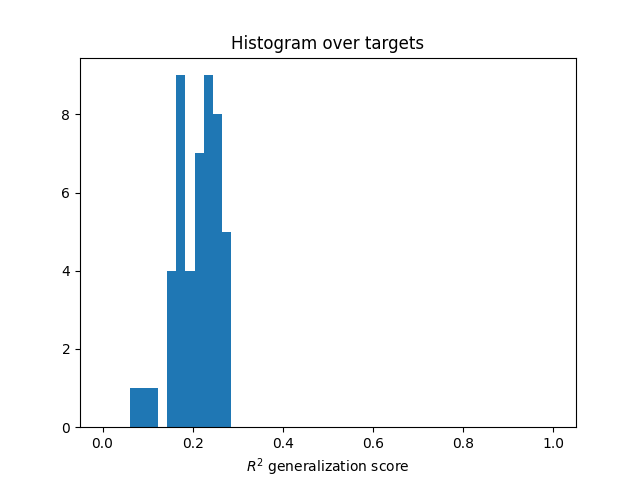
Compute the predictions on the test set
(requires the dual weights)
split = False
scores = predict_and_score_weighted_kernel_ridge(
    Ks_test, dual_weights, deltas, Y_test, split=split,
    n_targets_batch=n_targets_batch, score_func=r2_score_split)
scores = backend.to_numpy(scores)

plt.hist(scores, np.linspace(0, 1, 50))
plt.xlabel(r"$R^2$ generalization score")
plt.title("Histogram over targets")
plt.show()

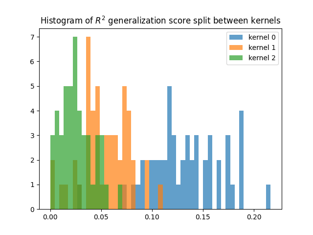
Compute the split predictions on the test set
(requires the dual weights)
Here we apply the dual weights on each kernel separately
(exp(deltas[i]) * kernel[i]), and we compute the R2 scores
(corrected for correlations) of each prediction.
split = True
scores_split = predict_and_score_weighted_kernel_ridge(
    Ks_test, dual_weights, deltas, Y_test, split=split,
    n_targets_batch=n_targets_batch, score_func=r2_score_split)
scores_split = backend.to_numpy(scores_split)

for kk, score in enumerate(scores_split):
    plt.hist(score, np.linspace(0, np.max(scores_split), 50), alpha=0.7,
             label="kernel %d" % kk)
plt.title(r"Histogram of $R^2$ generalization score split between kernels")
plt.legend()
plt.show()

Total running time of the script: (1 minutes 37.451 seconds)