Setup Google Colab#
In this script, we setup a Google Colab environment. This script will only work when run from Google Colab. You can skip it if you run the tutorials on your machine.
Note: This script will install all the required dependencies and download the data. It will take around 10 minutes to run, but you need to run it only once in your Colab session. If your Colab session is disconnected, you will need to run this script again.
Change runtime to use a GPU#
This tutorial is much faster when a GPU is available to run the computations. In Google Colab you can request access to a GPU by changing the runtime type. To do so, click the following menu options in Google Colab:
(Menu) “Runtime” -> “Change runtime type” -> “Hardware accelerator” -> “GPU”.
Install all required dependencies#
Uncomment and run the following cell to download the required packages.
#!git config --global user.email "you@example.com" && git config --global user.name "Your Name"
#!wget -O- http://neuro.debian.net/lists/jammy.us-ca.libre | sudo tee /etc/apt/sources.list.d/neurodebian.sources.list
#!apt-key adv --recv-keys --keyserver hkps://keyserver.ubuntu.com 0xA5D32F012649A5A9 > /dev/null
#!apt-get -qq update > /dev/null
#!apt-get install -qq inkscape git-annex-standalone > /dev/null
#!pip install -q voxelwise_tutorials
For the record, here is what each command does:
# - Set up an email and username to use git, git-annex, and datalad (required to download the data)
# - Add NeuroDebian to the package sources
# - Update the gpg keys to use NeuroDebian
# - Update the list of available packages
# - Install Inkscape to use more features from Pycortex, and install git-annex to download the data
# - Install the tutorial helper package, and all the required dependencies
try:
    import google.colab # noqa
    in_colab = True
except ImportError:
    in_colab = False
if not in_colab:
    raise RuntimeError("This script is only meant to be run from Google "
                       "Colab. You can skip it if you run the tutorials "
                       "on your machine.")
Now run the following cell to set up the environment variables for the tutorials and pycortex.
import os
os.environ['VOXELWISE_TUTORIALS_DATA'] = "/content"

import sklearn
sklearn.set_config(assume_finite=True)
Your Google Colab environment is now set up for the voxelwise tutorials.
%reset -f
Download the data set#
In this script, we download the data set from Wasabi or GIN. No account is required.
Note
This script will download approximately 2GB of data.
Cite this data set#
This tutorial is based on publicly available data published on GIN. If you publish any work using this data set, please cite the original publication [Huth et al., 2012], and the data set [Huth et al., 2022].
Download#
# path of the data directory
from voxelwise_tutorials.io import get_data_home
directory = get_data_home(dataset="shortclips")
print(directory)
We will only use the first subject in this tutorial, but you can run the same
analysis on the four other subjects. Uncomment the lines in DATAFILES to
download more subjects.
We also skip the stimuli files, since the dataset provides two preprocessed feature spaces to fit voxelwise encoding models without requiring the original stimuli.
from voxelwise_tutorials.io import download_datalad

DATAFILES = [
    "features/motion_energy.hdf",
    "features/wordnet.hdf",
    "mappers/S01_mappers.hdf",
    # "mappers/S02_mappers.hdf",
    # "mappers/S03_mappers.hdf",
    # "mappers/S04_mappers.hdf",
    # "mappers/S05_mappers.hdf",
    "responses/S01_responses.hdf",
    # "responses/S02_responses.hdf",
    # "responses/S03_responses.hdf",
    # "responses/S04_responses.hdf",
    # "responses/S05_responses.hdf",
    # "stimuli/test.hdf",
    # "stimuli/train_00.hdf",
    # "stimuli/train_01.hdf",
    # "stimuli/train_02.hdf",
    # "stimuli/train_03.hdf",
    # "stimuli/train_04.hdf",
    # "stimuli/train_05.hdf",
    # "stimuli/train_06.hdf",
    # "stimuli/train_07.hdf",
    # "stimuli/train_08.hdf",
    # "stimuli/train_09.hdf",
    # "stimuli/train_10.hdf",
    # "stimuli/train_11.hdf",
]

source = "https://gin.g-node.org/gallantlab/shortclips"

for datafile in DATAFILES:
    local_filename = download_datalad(datafile, destination=directory,
                                      source=source)
References#
T. Dupré la Tour, M. Eickenberg, A.O. Nunez-Elizalde, and J. L. Gallant. Feature-space selection with banded ridge regression. NeuroImage, 267:119728, 2022. doi:10.1016/j.neuroimage.2022.119728.
Trevor Hastie, Robert Tibshirani, and Jerome Friedman. The Elements of Statistical Learning. Springer New York, 2009.
A. Hsu, A. Borst, and F. E. Theunissen. Quantifying variability in neural responses and its application for the validation of model predictions. Network, 2004.
A. G. Huth, S. Nishimoto, A. T. Vu, T. Dupré la Tour, and J. L. Gallant. Gallant lab natural short clips 3t fMRI data. 2022. doi:10.12751/g-node.vy1zjd.
A. G. Huth, S. Nishimoto, A. T. Vu, and J. L. Gallant. A continuous semantic space describes the representation of thousands of object and action categories across the human brain. Neuron, 76(6):1210–1224, 2012.
S. Nishimoto, A. T. Vu, T. Naselaris, Y. Benjamini, B. Yu, and J. L. Gallant. Reconstructing visual experiences from brain activity evoked by natural movies. Current Biology, 21(19):1641–1646, 2011.
A. O. Nunez-Elizalde, A. G. Huth, and J. L. Gallant. Voxelwise encoding models with non-spherical multivariate normal priors. Neuroimage, 197:482–492, 2019.
M. Sahani and J. Linden. How linear are auditory cortical responses? Adv. Neural Inf. Process. Syst., 2002.
C. Saunders, A. Gammerman, and V. Vovk. Ridge regression learning algorithm in dual variables. 1998.
O. Schoppe, N. S. Harper, B. Willmore, A. King, and J. Schnupp. Measuring the performance of neural models. Front. Comput. Neurosci., 2016.
%reset -f
Compute the explainable variance#
Before fitting any voxelwise model to fMRI responses, it is good practice to quantify the amount of signal in the test set that can be predicted by an encoding model. This quantity is called the explainable variance.
The measured signal can be decomposed into a sum of two components: the stimulus-dependent signal and noise. If we present the same stimulus multiple times and we record brain activity for each repetition, the stimulus-dependent signal will be the same across repetitions while the noise will vary across repetitions. In the Voxelwise Encoding Model framework, the features used to model brain activity are the same for each repetition of the stimulus. Thus, encoding models will predict only the repeatable stimulus-dependent signal.
The stimulus-dependent signal can be estimated by taking the mean of brain responses over repeats of the same stimulus or experiment. The variance of the estimated stimulus-dependent signal, which we call the explainable variance, is proportional to the maximum prediction accuracy that can be obtained by a voxelwise encoding model in the test set.
Mathematically, let \(y_i, i = 1 \dots N\) be the measured signal in a voxel for each of the \(N\) repetitions of the same stimulus and \(\bar{y} = \frac{1}{N}\sum_{i=1}^Ny_i\) the average brain response across repetitions. For each repeat, we define the residual timeseries between brain response and average brain response as \(r_i = y_i - \bar{y}\). The explainable variance (EV) is estimated as
In the literature, the explainable variance is also known as the signal power.
For more information, see [Hsu et al., 2004, Sahani and Linden, 2002, Schoppe et al., 2016].
Path of the data directory#
from voxelwise_tutorials.io import get_data_home

directory = get_data_home(dataset="shortclips")
print(directory)
# modify to use another subject
subject = "S01"
Compute the explainable variance#
import numpy as np
from voxelwise_tutorials.io import load_hdf5_array
First, we load the fMRI responses on the test set, which contains brain responses to ten (10) repeats of the same stimulus.
import os

file_name = os.path.join(directory, 'responses', f'{subject}_responses.hdf')
Y_test = load_hdf5_array(file_name, key="Y_test")
print("(n_repeats, n_samples_test, n_voxels) =", Y_test.shape)
Then, we compute the explainable variance for each voxel.
from voxelwise_tutorials.utils import explainable_variance

ev = explainable_variance(Y_test)
print("(n_voxels,) =", ev.shape)
To better understand the concept of explainable variance, we can plot the measured signal in a voxel with high explainable variance…
import matplotlib.pyplot as plt

voxel_1 = np.argmax(ev)
time = np.arange(Y_test.shape[1]) * 2  # one time point every 2 seconds
plt.figure(figsize=(10, 3))
plt.plot(time, Y_test[:, :, voxel_1].T, color='C0', alpha=0.5)
plt.plot(time, Y_test[:, :, voxel_1].mean(0), color='C1', label='average')
plt.xlabel("Time (sec)")
plt.title("Voxel with large explainable variance (%.2f)" % ev[voxel_1])
plt.yticks([])
plt.legend()
plt.tight_layout()
plt.show()
… and in a voxel with low explainable variance.
voxel_2 = np.argmin(ev)
plt.figure(figsize=(10, 3))
plt.plot(time, Y_test[:, :, voxel_2].T, color='C0', alpha=0.5)
plt.plot(time, Y_test[:, :, voxel_2].mean(0), color='C1', label='average')
plt.xlabel("Time (sec)")
plt.title("Voxel with low explainable variance (%.2f)" % ev[voxel_2])
plt.yticks([])
plt.legend()
plt.tight_layout()
plt.show()
We can also plot the distribution of explainable variance over voxels.
plt.hist(ev, bins=np.linspace(0, 1, 100), log=True, histtype='step')
plt.xlabel("Explainable variance")
plt.ylabel("Number of voxels")
plt.title('Histogram of explainable variance')
plt.grid('on')
plt.show()
We see that many voxels have low explainable variance. This is expected, since many voxels are not driven by a visual stimulus, and their response changes over repeats of the same stimulus. We also see that some voxels have high explainable variance (around 0.7). The responses in these voxels are highly consistent across repetitions of the same stimulus. Thus, they are good targets for encoding models.
Map to subject flatmap#
To better understand the distribution of explainable variance, we map the
values to the subject brain. This can be done with pycortex, which can create interactive 3D
viewers to be displayed in any modern browser. pycortex can also display
flattened maps of the cortical surface to visualize the entire cortical
surface at once.
Here, we do not share the anatomical information of the subjects for privacy concerns. Instead, we provide two mappers:
to map the voxels to a (subject-specific) flatmap
to map the voxels to the Freesurfer average cortical surface (“fsaverage”)
The first mapper is 2D matrix of shape (n_pixels, n_voxels) that maps each
voxel to a set of pixel in a flatmap. The matrix is efficiently stored in a
scipy sparse CSR matrix. The function plot_flatmap_from_mapper
provides an example of how to use the mapper and visualize the flatmap.
from voxelwise_tutorials.viz import plot_flatmap_from_mapper

mapper_file = os.path.join(directory, 'mappers', f'{subject}_mappers.hdf')
plot_flatmap_from_mapper(ev, mapper_file, vmin=0, vmax=0.7)
plt.show()
This figure is a flattened map of the cortical surface. A number of regions
of interest (ROIs) have been labeled to ease interpretation. If you have
never seen such a flatmap, we recommend taking a look at a pycortex brain
viewer, which displays
the brain in 3D. In this viewer, press “I” to inflate the brain, “F” to
flatten the surface, and “R” to reset the view (or use the surface/unfold
cursor on the right menu). Press “H” for a list of all keyboard shortcuts.
This viewer should help you understand the correspondence between the flatten
and the folded cortical surface of the brain.
On this flatmap, we can see that the explainable variance is mainly located in the visual cortex, in early visual regions like V1, V2, V3, or in higher-level regions like EBA, FFA or IPS. This is expected since this dataset contains responses to a visual stimulus.
Map to “fsaverage”#
The second mapper we provide maps the voxel data to a Freesurfer
average surface (“fsaverage”), that can be used in pycortex.
First, let’s download the “fsaverage” surface.
import cortex

surface = "fsaverage"

if not hasattr(cortex.db, surface):
    cortex.utils.download_subject(subject_id=surface,
                                  pycortex_store=cortex.db.filestore)
    cortex.db.reload_subjects()  # force filestore reload
    assert hasattr(cortex.db, surface)
Then, we load the “fsaverage” mapper. The mapper is a matrix of shape
(n_vertices, n_voxels), which maps each voxel to some vertices in the
fsaverage surface. It is stored as a sparse CSR matrix. The mapper is applied
with a dot product @ (equivalent to np.dot).
from voxelwise_tutorials.io import load_hdf5_sparse_array

voxel_to_fsaverage = load_hdf5_sparse_array(mapper_file,
                                            key='voxel_to_fsaverage')
ev_projected = voxel_to_fsaverage @ ev
print("(n_vertices,) =", ev_projected.shape)
We can then create a Vertex object in pycortex, containing the
projected data. This object can be used either in a pycortex interactive
3D viewer, or in a matplotlib figure showing only the flatmap.
vertex = cortex.Vertex(ev_projected, surface, vmin=0, vmax=0.7, cmap='viridis')
To start an interactive 3D viewer in the browser, we can use the webshow
function in pycortex. (Note that this method works only if you are running the
notebooks locally.) You can start an interactive 3D viewer by changing
run_webshow to True and running the following cell.
run_webshow = False
if run_webshow:
    cortex.webshow(vertex, open_browser=False, port=8050)
Alternatively, to plot a flatmap in a matplotlib figure, use the
quickshow function.
(This function requires Inkscape to be installed. The rest of the tutorial does not use this function, so feel free to ignore.)
from cortex.testing_utils import has_installed

fig = cortex.quickshow(vertex, colorbar_location='right',
                       with_rois=has_installed("inkscape"))
plt.show()
References#
T. Dupré la Tour, M. Eickenberg, A.O. Nunez-Elizalde, and J. L. Gallant. Feature-space selection with banded ridge regression. NeuroImage, 267:119728, 2022. doi:10.1016/j.neuroimage.2022.119728.
Trevor Hastie, Robert Tibshirani, and Jerome Friedman. The Elements of Statistical Learning. Springer New York, 2009.
A. Hsu, A. Borst, and F. E. Theunissen. Quantifying variability in neural responses and its application for the validation of model predictions. Network, 2004.
A. G. Huth, S. Nishimoto, A. T. Vu, T. Dupré la Tour, and J. L. Gallant. Gallant lab natural short clips 3t fMRI data. 2022. doi:10.12751/g-node.vy1zjd.
A. G. Huth, S. Nishimoto, A. T. Vu, and J. L. Gallant. A continuous semantic space describes the representation of thousands of object and action categories across the human brain. Neuron, 76(6):1210–1224, 2012.
S. Nishimoto, A. T. Vu, T. Naselaris, Y. Benjamini, B. Yu, and J. L. Gallant. Reconstructing visual experiences from brain activity evoked by natural movies. Current Biology, 21(19):1641–1646, 2011.
A. O. Nunez-Elizalde, A. G. Huth, and J. L. Gallant. Voxelwise encoding models with non-spherical multivariate normal priors. Neuroimage, 197:482–492, 2019.
M. Sahani and J. Linden. How linear are auditory cortical responses? Adv. Neural Inf. Process. Syst., 2002.
C. Saunders, A. Gammerman, and V. Vovk. Ridge regression learning algorithm in dual variables. 1998.
O. Schoppe, N. S. Harper, B. Willmore, A. King, and J. Schnupp. Measuring the performance of neural models. Front. Comput. Neurosci., 2016.
%reset -f
Fit a voxelwise encoding model with WordNet features#
In this example, we model the fMRI responses with semantic “wordnet” features, manually annotated on each frame of the movie stimulus. The model is a regularized linear regression model, known as ridge regression. Since this model is used to predict brain activity from the stimulus, it is called a (voxelwise) encoding model.
This example reproduces part of the analysis described in Huth et al. [2012]. See the original publication for more details about the experiment, the wordnet features, along with more results and more discussions.
WordNet features: The features used in this example are semantic labels manually annotated on each frame of the movie stimulus. The semantic labels include nouns (such as “woman”, “car”, or “building”) and verbs (such as “talking”, “touching”, or “walking”), for a total of 1705 distinct category labels. To interpret our model, labels can be organized in a graph of semantic relationship based on the WordNet dataset.
Summary: We first concatenate the features with multiple temporal delays to account for the slow hemodynamic response. We then use linear regression to fit a predictive model of brain activity. The linear regression is regularized to improve robustness to correlated features and to improve generalization performance. The optimal regularization hyperparameter is selected over a grid-search with cross-validation. Finally, the model generalization performance is evaluated on a held-out test set, comparing the model predictions to the corresponding ground-truth fMRI responses.
Note
It should take less than 5 minutes to run the model fitting in this tutorial on a GPU. If you are using a CPU, it may take longer.
Path of the data directory#
from voxelwise_tutorials.io import get_data_home
directory = get_data_home(dataset="shortclips")
print(directory)
# modify to use another subject
subject = "S01"
Load the data#
We first load the fMRI responses. These responses have been preprocessed as
described in Huth et al. [2012]. The data is separated into a training set Y_train and a
testing set Y_test. The training set is used for fitting models, and
selecting the best models and hyperparameters. The test set is later used
to estimate the generalization performance of the selected model. The
test set contains multiple repetitions of the same experiment to estimate
an upper bound of the model prediction accuracy (cf. previous example).
import os
import numpy as np
from voxelwise_tutorials.io import load_hdf5_array

file_name = os.path.join(directory, "responses", f"{subject}_responses.hdf")
Y_train = load_hdf5_array(file_name, key="Y_train")
Y_test = load_hdf5_array(file_name, key="Y_test")

print("(n_samples_train, n_voxels) =", Y_train.shape)
print("(n_repeats, n_samples_test, n_voxels) =", Y_test.shape)
Before fitting an encoding model, the fMRI responses are typically z-scored over time. This normalization step is performed for two reasons. First, the regularized regression methods used to estimate encoding models generally assume the data to be normalized [Hastie et al., 2009]. Second, the temporal mean and standard deviation of a voxel are typically considered uninformative in fMRI because they can vary due to factors unrelated to the task, such as differences in signal-to-noise ratio (SNR).
To preserve each run independent from the others, we z-score each run separately.
from scipy.stats import zscore
from voxelwise_tutorials.utils import zscore_runs

# indice of first sample of each run
run_onsets = load_hdf5_array(file_name, key="run_onsets")
print(run_onsets)

# zscore each training run separately
Y_train = zscore_runs(Y_train, run_onsets)
# zscore each test run separately
Y_test = zscore(Y_test, axis=1)
If we repeat an experiment multiple times, part of the fMRI responses might change. However the modeling features do not change over the repeats, so the voxelwise encoding model will predict the same signal for each repeat. To have an upper bound of the model prediction accuracy, we keep only the repeatable part of the signal by averaging the test repeats.
Y_test = Y_test.mean(0)
# We need to zscore the test data again, because we took the mean across repetitions.
Y_test = zscore(Y_test, axis=0)

print("(n_samples_test, n_voxels) =", Y_test.shape)
We fill potential NaN (not-a-number) values with zeros.
Y_train = np.nan_to_num(Y_train)
Y_test = np.nan_to_num(Y_test)
Then, we load the semantic “wordnet” features, extracted from the stimulus at
each time point. The features corresponding to the training set are noted
X_train, and the features corresponding to the test set are noted
X_test.
feature_space = "wordnet"

file_name = os.path.join(directory, "features", f"{feature_space}.hdf")
X_train = load_hdf5_array(file_name, key="X_train")
X_test = load_hdf5_array(file_name, key="X_test")

print("(n_samples_train, n_features) =", X_train.shape)
print("(n_samples_test, n_features) =", X_test.shape)
Define the cross-validation scheme#
To select the best hyperparameter through cross-validation, we must define a cross-validation splitting scheme. Because fMRI time-series are autocorrelated in time, we should preserve as much as possible the temporal correlation. In other words, because consecutive time samples are correlated, we should not put one time sample in the training set and the immediately following time sample in the validation set. Thus, we define here a leave-one-run-out cross-validation split that keeps each recording run intact.
We define a cross-validation splitter, compatible with scikit-learn API.
from sklearn.model_selection import check_cv
from voxelwise_tutorials.utils import generate_leave_one_run_out

n_samples_train = X_train.shape[0]
cv = generate_leave_one_run_out(n_samples_train, run_onsets)
cv = check_cv(cv)  # copy the cross-validation splitter into a reusable list
Define the model#
Now, let’s define the model pipeline.
With regularized linear regression models, it is generally recommended to normalize (z-score) both the responses and the features before fitting the model [Hastie et al., 2009]. Z-scoring corresponds to removing the temporal mean and dividing by the temporal standard deviation. We already z-scored the fMRI responses after loading them, so now we need to specify in the model how to deal with the features.
We first center the features, since we will not use an intercept. The mean value in fMRI recording is non-informative, so each run is detrended and demeaned independently, and we do not need to predict an intercept value in the linear model.
For this particular dataset and example, we do not normalize by the standard deviation of each feature. If the features are extracted in a consistent way from the stimulus, their relative scale is meaningful. Normalizing them independently from each other would remove this information. Moreover, the wordnet features are one-hot-encoded, which means that each feature is either present (1) or not present (0) in each sample. Normalizing one-hot-encoded features is not recommended, since it would scale disproportionately the infrequent features.
from sklearn.preprocessing import StandardScaler
scaler = StandardScaler(with_mean=True, with_std=False)
Then we concatenate the features with multiple delays to account for the
hemodynamic response. Due to neurovascular coupling, the recorded BOLD signal
is delayed in time with respect to the stimulus onset. With different delayed
versions of the features, the linear regression model will weigh each delayed
feature with a different weight to maximize the predictions. With a sample
every 2 seconds, we typically use 4 delays [1, 2, 3, 4] to cover the
hemodynamic response peak. In the next example, we further describe this
hemodynamic response estimation.
from voxelwise_tutorials.delayer import Delayer
delayer = Delayer(delays=[1, 2, 3, 4])
Finally, we use a ridge regression model. Ridge regression is a linear
regression with L2 regularization. The L2 regularization improves robustness
to correlated features and improves generalization performance. The L2
regularization is controlled by a hyperparameter alpha that needs to be
tuned for each dataset. This regularization hyperparameter is usually
selected over a grid search with cross-validation, selecting the
hyperparameter that maximizes the predictive performances on the validation
set. See the previous example for more details about ridge regression and
hyperparameter selection.
For computational reasons, when the number of features is larger than the number of samples, it is more efficient to solve ridge regression using the (equivalent) dual formulation [Saunders et al., 1998]. This dual formulation is equivalent to kernel ridge regression with a linear kernel. Here, we have 3600 training samples, and 1705 * 4 = 6820 features (we multiply by 4 since we use 4 time delays), therefore it is more efficient to use kernel ridge regression.
With one target, we could directly use the pipeline in scikit-learn’s
GridSearchCV, to select the optimal regularization hyperparameter
(alpha) over cross-validation. However, GridSearchCV can only
optimize a single score across all voxels (targets). Thus, in the
multiple-target case, GridSearchCV can only optimize (for example) the
mean score over targets. Here, we want to find a different optimal
hyperparameter per target/voxel, so we use the package himalaya which implements a
scikit-learn compatible estimator KernelRidgeCV, with hyperparameter
selection independently on each target.
from himalaya.kernel_ridge import KernelRidgeCV
himalaya implements different computational backends,
including two backends that use GPU for faster computations. The two
available GPU backends are “torch_cuda” and “cupy”. (Each backend is only
available if you installed the corresponding package with CUDA enabled. Check
the pytorch/cupy documentation for install instructions.)
Here we use the “torch_cuda” backend, but if the import fails we continue with the default “numpy” backend. The “numpy” backend is expected to be slower since it only uses the CPU.
from himalaya.backend import set_backend
backend = set_backend("torch_cuda", on_error="warn")
print(backend)
To speed up model fitting on GPU, we use single precision float numbers. (This step probably does not change significantly the performances on non-GPU backends.)
X_train = X_train.astype("float32")
X_test = X_test.astype("float32")
Since the scale of the regularization hyperparameter alpha is unknown, we
use a large logarithmic range, and we will check after the fit that best
hyperparameters are not all on one range edge.
alphas = np.logspace(1, 20, 20)
We also indicate some batch sizes to limit the GPU memory.
kernel_ridge_cv = KernelRidgeCV(
    alphas=alphas, cv=cv,
    solver_params=dict(n_targets_batch=500, n_alphas_batch=5,
                       n_targets_batch_refit=100))
Finally, we use a scikit-learn Pipeline to link the different steps
together. A Pipeline can be used as a regular estimator, calling
pipeline.fit, pipeline.predict, etc. Using a Pipeline can be
useful to clarify the different steps, avoid cross-validation mistakes, or
automatically cache intermediate results. See the scikit-learn
documentation for
more information.
from sklearn.pipeline import make_pipeline
pipeline = make_pipeline(
    scaler,
    delayer,
    kernel_ridge_cv,
)
We can display the scikit-learn pipeline with an HTML diagram.
from sklearn import set_config
set_config(display='diagram')  # requires scikit-learn 0.23
pipeline
Fit the model#
We fit on the training set..
_ = pipeline.fit(X_train, Y_train)
..and score on the test set. Here the scores are the \(R^2\) scores, with values in \(]-\infty, 1]\). A value of \(1\) means the predictions are perfect.
Note that since himalaya is implementing multiple-targets
models, the score method differs from scikit-learn API and returns
one score per target/voxel.
scores = pipeline.score(X_test, Y_test)
print("(n_voxels,) =", scores.shape)
If we fit the model on GPU, scores are returned on GPU using an array object
specific to the backend we used (such as a torch.Tensor). Thus, we need to
move them into numpy arrays on CPU, to be able to use them for example in
a matplotlib figure.
scores = backend.to_numpy(scores)
Plot the model prediction accuracy#
To visualize the model prediction accuracy, we can plot it for each voxel on a flattened surface of the brain. To do so, we use a mapper that is specific to the each subject’s brain. (Check previous example to see how to use the mapper to Freesurfer average surface.)
import matplotlib.pyplot as plt
from voxelwise_tutorials.viz import plot_flatmap_from_mapper

mapper_file = os.path.join(directory, "mappers", f"{subject}_mappers.hdf")
ax = plot_flatmap_from_mapper(scores, mapper_file, vmin=0, vmax=0.4)
plt.show()
We can see that the “wordnet” features successfully predict part of the measured brain activity, with \(R^2\) scores as high as 0.4. Note that these scores are generalization scores, since they are computed on a test set that was not used during model fitting. Since we fitted a model independently in each voxel, we can inspect the generalization performances at the best available spatial resolution: individual voxels.
The best-predicted voxels are located in visual semantic areas like EBA, or FFA. This is expected since the wordnet features encode semantic information about the visual stimulus. For more discussions about these results, we refer the reader to the original publication [Huth et al., 2012].
Plot the selected hyperparameters#
Since the scale of alphas is unknown, we plot the optimal alphas selected by the solver over cross-validation. This plot is helpful to refine the alpha grid if the range is too small or too large.
Note that some voxels might be at the maximum regularization value in the grid search. These are voxels where the model has no predictive power, thus the optimal regularization parameter is large to lead to a prediction equal to zero. We do not need to extend the alpha range for these voxels.
from himalaya.viz import plot_alphas_diagnostic
best_alphas = backend.to_numpy(pipeline[-1].best_alphas_)
plot_alphas_diagnostic(best_alphas=best_alphas, alphas=alphas)
plt.show()
Visualize the regression coefficients#
Here, we go back to the main model on all voxels. Since our model is linear, we can use the (primal) regression coefficients to interpret the model. The basic intuition is that the model will use larger coefficients on features that have more predictive power.
Since we know the meaning of each feature, we can interpret the large regression coefficients. In the case of wordnet features, we can even build a graph that represents the features that are linked by a semantic relationship.
We first get the (primal) ridge regression coefficients from the fitted model.
primal_coef = pipeline[-1].get_primal_coef()
primal_coef = backend.to_numpy(primal_coef)
print("(n_delays * n_features, n_voxels) =", primal_coef.shape)
Because the ridge model allows a different regularization per voxel, the regression coefficients may have very different scales. In turn, these different scales can introduce a bias in the interpretation, focusing the attention disproportionately on voxels fitted with the lowest alpha. To address this issue, we rescale the regression coefficient to have a norm equal to the square-root of the \(R^2\) scores. We found empirically that this rescaling best matches results obtained with a regularization shared across voxels. This rescaling also removes the need to select only best performing voxels, because voxels with low prediction accuracies are rescaled to have a low norm.
primal_coef /= np.linalg.norm(primal_coef, axis=0)[None]
primal_coef *= np.sqrt(np.maximum(0, scores))[None]
Then, we aggregate the coefficients across the different delays.
# split the ridge coefficients per delays
delayer = pipeline.named_steps['delayer']
primal_coef_per_delay = delayer.reshape_by_delays(primal_coef, axis=0)
print("(n_delays, n_features, n_voxels) =", primal_coef_per_delay.shape)
del primal_coef

# average over delays
average_coef = np.mean(primal_coef_per_delay, axis=0)
print("(n_features, n_voxels) =", average_coef.shape)
del primal_coef_per_delay
Even after averaging over delays, the coefficient matrix is still too large to interpret it. Therefore, we use principal component analysis (PCA) to reduce the dimensionality of the matrix.
from sklearn.decomposition import PCA

pca = PCA(n_components=4)
pca.fit(average_coef.T)
components = pca.components_
print("(n_components, n_features) =", components.shape)
We can check the ratio of explained variance by each principal component. We see that the first four components already explain a large part of the coefficients variance.
print("PCA explained variance =", pca.explained_variance_ratio_)
Similarly to Huth et al. [2012], we correct the coefficients of features linked by a
semantic relationship. When building the wordnet features, if a frame was
labeled with wolf, the authors automatically added the semantically linked
categories canine, carnivore, placental mammal, mammal, vertebrate,
chordate, organism, and whole. The authors thus argue that the same
correction needs to be done on the coefficients.
from voxelwise_tutorials.wordnet import load_wordnet
from voxelwise_tutorials.wordnet import correct_coefficients
_, wordnet_categories = load_wordnet(directory=directory)
components = correct_coefficients(components.T, wordnet_categories).T
components -= components.mean(axis=1)[:, None]
components /= components.std(axis=1)[:, None]
Finally, we plot the first principal component on the wordnet graph. In such
graph, edges indicate “is a” relationships (e.g. an athlete “is a”
person). Each marker represents a single noun (circle) or verb (square).
The area of each marker indicates the principal component magnitude, and the
color indicates the sign (red is positive, blue is negative).
from voxelwise_tutorials.wordnet import plot_wordnet_graph
from voxelwise_tutorials.wordnet import apply_cmap

first_component = components[0]
node_sizes = np.abs(first_component)
node_colors = apply_cmap(first_component, vmin=-2, vmax=2, cmap='coolwarm',
                         n_colors=2)

plot_wordnet_graph(node_colors=node_colors, node_sizes=node_sizes)
plt.show()
According to Huth et al. [2012], “this principal component distinguishes
between categories with high stimulus energy (e.g. moving objects like
person and vehicle) and those with low stimulus energy (e.g. stationary
objects like sky and city)”.
In this example, because we use only a single subject and we perform a different voxel selection, our result is slightly different than in the original publication. We also use a different regularization parameter in each voxel, while in Huth et al. [2012] all voxels had the same regularization parameter. However, we do not aim at reproducing exactly the results of the original publication, but we rather describe the general approach.
To project the principal component on the cortical surface, we first need to use the fitted PCA to transform the primal weights of all voxels.
# transform with the fitted PCA
average_coef_transformed = pca.transform(average_coef.T).T
print("(n_components, n_voxels) =", average_coef_transformed.shape)
del average_coef

# We make sure vmin = -vmax, so that the colormap is centered on 0.
vmax = np.percentile(np.abs(average_coef_transformed), 99.9)

# plot the primal weights projected on the first principal component.
ax = plot_flatmap_from_mapper(average_coef_transformed[0], mapper_file,
                              vmin=-vmax, vmax=vmax, cmap='coolwarm')
plt.show()
This flatmap shows in which brain regions the model has the largest projection on the first component. Again, this result is different from the one in Huth et al. [2012], and should only be considered as reproducing the general approach.
Following the analyses in the original publication, we also plot the next three principal components on the wordnet graph, mapping the three vectors to RGB colors.
from voxelwise_tutorials.wordnet import scale_to_rgb_cube

next_three_components = components[1:4].T
node_sizes = np.linalg.norm(next_three_components, axis=1)
node_colors = scale_to_rgb_cube(next_three_components)
print("(n_nodes, n_channels) =", node_colors.shape)

plot_wordnet_graph(node_colors=node_colors, node_sizes=node_sizes)
plt.show()
According to Huth et al. [2012], “this graph shows that categories thought to be semantically related (e.g. athletes and walking) are represented similarly in the brain”.
Finally, we project these principal components on the cortical surface.
from voxelwise_tutorials.viz import plot_3d_flatmap_from_mapper

voxel_colors = scale_to_rgb_cube(average_coef_transformed[1:4].T, clip=3).T
print("(n_channels, n_voxels) =", voxel_colors.shape)

ax = plot_3d_flatmap_from_mapper(
    voxel_colors[0], voxel_colors[1], voxel_colors[2],
    mapper_file=mapper_file,
    vmin=0, vmax=1, vmin2=0, vmax2=1, vmin3=0, vmax3=1
)
plt.show()
Again, our results are different from the ones in Huth et al. [2012], for the same reasons mentioned earlier.
References#
T. Dupré la Tour, M. Eickenberg, A.O. Nunez-Elizalde, and J. L. Gallant. Feature-space selection with banded ridge regression. NeuroImage, 267:119728, 2022. doi:10.1016/j.neuroimage.2022.119728.
Trevor Hastie, Robert Tibshirani, and Jerome Friedman. The Elements of Statistical Learning. Springer New York, 2009.
A. Hsu, A. Borst, and F. E. Theunissen. Quantifying variability in neural responses and its application for the validation of model predictions. Network, 2004.
A. G. Huth, S. Nishimoto, A. T. Vu, T. Dupré la Tour, and J. L. Gallant. Gallant lab natural short clips 3t fMRI data. 2022. doi:10.12751/g-node.vy1zjd.
A. G. Huth, S. Nishimoto, A. T. Vu, and J. L. Gallant. A continuous semantic space describes the representation of thousands of object and action categories across the human brain. Neuron, 76(6):1210–1224, 2012.
S. Nishimoto, A. T. Vu, T. Naselaris, Y. Benjamini, B. Yu, and J. L. Gallant. Reconstructing visual experiences from brain activity evoked by natural movies. Current Biology, 21(19):1641–1646, 2011.
A. O. Nunez-Elizalde, A. G. Huth, and J. L. Gallant. Voxelwise encoding models with non-spherical multivariate normal priors. Neuroimage, 197:482–492, 2019.
M. Sahani and J. Linden. How linear are auditory cortical responses? Adv. Neural Inf. Process. Syst., 2002.
C. Saunders, A. Gammerman, and V. Vovk. Ridge regression learning algorithm in dual variables. 1998.
O. Schoppe, N. S. Harper, B. Willmore, A. King, and J. Schnupp. Measuring the performance of neural models. Front. Comput. Neurosci., 2016.
%reset -f
Fit a voxelwise encoding model with motion-energy features#
In this example, we model the fMRI responses with motion-energy features extracted from the movie stimulus. The model is a regularized linear regression model.
This tutorial reproduces part of the analysis described in Nishimoto et al. [2011]. See the original publication for more details about the experiment, the motion-energy features, along with more results and more discussions.
Motion-energy features: Motion-energy features result from filtering a video stimulus with spatio-temporal Gabor filters. A pyramid of filters is used to compute the motion-energy features at multiple spatial and temporal scales. Motion-energy features were introduced in Nishimoto et al. [2011]. The downloaded dataset contains the pre-computed motion-energy features for the movie stimulus used in the experiment. You can see how to extract these motion-energy features in the Extract motion-energy features tutorial.
Summary: As in the previous example, we first concatenate the features with multiple delays, to account for the slow hemodynamic response. A linear regression model then weights each delayed feature with a different weight, to build a predictive model of BOLD activity. Again, the linear regression is regularized to improve robustness to correlated features and to improve generalization. The optimal regularization hyperparameter is selected independently on each voxel over a grid-search with cross-validation. Finally, the model generalization performance is evaluated on a held-out test set, comparing the model predictions with the ground-truth fMRI responses.
Note
It should take less than 5 minutes to run the model fitting in this tutorial on a GPU. If you are using a CPU, it may take longer.
Path of the data directory#
from voxelwise_tutorials.io import get_data_home
directory = get_data_home(dataset="shortclips")
print(directory)
# modify to use another subject
subject = "S01"
Load the data#
We first load and normalize the fMRI responses.
import os
import numpy as np
from scipy.stats import zscore
from voxelwise_tutorials.io import load_hdf5_array
from voxelwise_tutorials.utils import zscore_runs

file_name = os.path.join(directory, "responses", f"{subject}_responses.hdf")
Y_train = load_hdf5_array(file_name, key="Y_train")
Y_test = load_hdf5_array(file_name, key="Y_test")

print("(n_samples_train, n_voxels) =", Y_train.shape)
print("(n_repeats, n_samples_test, n_voxels) =", Y_test.shape)

# indice of first sample of each run
run_onsets = load_hdf5_array(file_name, key="run_onsets")

# zscore each training run separately
Y_train = zscore_runs(Y_train, run_onsets)
# zscore each test run separately
Y_test = zscore(Y_test, axis=1)
We average the test repeats, to remove the non-repeatable part of fMRI responses, and normalize the average across repeats.
Y_test = Y_test.mean(0)
Y_test = zscore(Y_test, axis=0)

print("(n_samples_test, n_voxels) =", Y_test.shape)
We fill potential NaN (not-a-number) values with zeros.
Y_train = np.nan_to_num(Y_train)
Y_test = np.nan_to_num(Y_test)
Then we load the precomputed “motion-energy” features.
feature_space = "motion_energy"
file_name = os.path.join(directory, "features", f"{feature_space}.hdf")
X_train = load_hdf5_array(file_name, key="X_train")
X_test = load_hdf5_array(file_name, key="X_test")

print("(n_samples_train, n_features) =", X_train.shape)
print("(n_samples_test, n_features) =", X_test.shape)
Define the cross-validation scheme#
We define the same leave-one-run-out cross-validation split as in the previous example.
from sklearn.model_selection import check_cv
from voxelwise_tutorials.utils import generate_leave_one_run_out

# indice of first sample of each run
run_onsets = load_hdf5_array(file_name, key="run_onsets")
print(run_onsets)
We define a cross-validation splitter, compatible with scikit-learn API.
n_samples_train = X_train.shape[0]
cv = generate_leave_one_run_out(n_samples_train, run_onsets)
cv = check_cv(cv)  # copy the cross-validation splitter into a reusable list
Define the model#
We define the same model as in the previous example. See the previous example for more details about the model definition.
from sklearn.pipeline import make_pipeline
from sklearn.preprocessing import StandardScaler
from voxelwise_tutorials.delayer import Delayer
from himalaya.kernel_ridge import KernelRidgeCV
from himalaya.backend import set_backend
backend = set_backend("torch_cuda", on_error="warn")

X_train = X_train.astype("float32")
X_test = X_test.astype("float32")

alphas = np.logspace(1, 20, 20)

pipeline = make_pipeline(
    StandardScaler(with_mean=True, with_std=False),
    Delayer(delays=[1, 2, 3, 4]),
    KernelRidgeCV(
        alphas=alphas, cv=cv,
        solver_params=dict(n_targets_batch=500, n_alphas_batch=5,
                           n_targets_batch_refit=100)),
)
from sklearn import set_config
set_config(display='diagram')  # requires scikit-learn 0.23
pipeline
Fit the model#
We fit on the train set, and score on the test set.
pipeline.fit(X_train, Y_train)

scores_motion_energy = pipeline.score(X_test, Y_test)
scores_motion_energy = backend.to_numpy(scores_motion_energy)

print("(n_voxels,) =", scores_motion_energy.shape)
Plot the model performances#
The performances are computed using the \(R^2\) scores.
import matplotlib.pyplot as plt
from voxelwise_tutorials.viz import plot_flatmap_from_mapper

mapper_file = os.path.join(directory, "mappers", f"{subject}_mappers.hdf")
ax = plot_flatmap_from_mapper(scores_motion_energy, mapper_file, vmin=0,
                              vmax=0.5)
plt.show()
The motion-energy features lead to large generalization scores in the early visual cortex (V1, V2, V3, …). For more discussions about these results, we refer the reader to the original publication [Nishimoto et al., 2011].
Compare with the wordnet model#
Interestingly, the motion-energy model performs well in different brain regions than the semantic “wordnet” model fitted in the previous example. To compare the two models, we first need to fit again the wordnet model.
feature_space = "wordnet"
file_name = os.path.join(directory, "features", f"{feature_space}.hdf")
X_train = load_hdf5_array(file_name, key="X_train")
X_test = load_hdf5_array(file_name, key="X_test")

X_train = X_train.astype("float32")
X_test = X_test.astype("float32")
We can create an unfitted copy of the pipeline with the clone function,
or simply call fit again if we do not need to reuse the previous model.
if False:
    from sklearn.base import clone
    pipeline_wordnet = clone(pipeline)
    pipeline_wordnet
pipeline.fit(X_train, Y_train)
scores_wordnet = pipeline.score(X_test, Y_test)
scores_wordnet = backend.to_numpy(scores_wordnet)

ax = plot_flatmap_from_mapper(scores_wordnet, mapper_file, vmin=0,
                              vmax=0.5)
plt.show()
We can also plot the comparison of model prediction accuracies with a 2D histogram. All ~70k voxels are represented in this histogram, where the diagonal corresponds to identical prediction accuracy for both models. A distribution deviating from the diagonal means that one model has better predictive performance than the other.
from voxelwise_tutorials.viz import plot_hist2d

ax = plot_hist2d(scores_wordnet, scores_motion_energy)
ax.set(title='Generalization R2 scores', xlabel='semantic wordnet model',
       ylabel='motion energy model')
plt.show()
Interestingly, the well predicted voxels are different in the two models. To further describe these differences, we can plot both performances on the same flatmap, using a 2D colormap.
from voxelwise_tutorials.viz import plot_2d_flatmap_from_mapper

mapper_file = os.path.join(directory, "mappers", f"{subject}_mappers.hdf")
ax = plot_2d_flatmap_from_mapper(scores_wordnet, scores_motion_energy,
                                 mapper_file, vmin=0, vmax=0.25, vmin2=0,
                                 vmax2=0.5, label_1="wordnet",
                                 label_2="motion energy")
plt.show()
The blue regions are well predicted by the motion-energy features, the orange regions are well predicted by the wordnet features, and the white regions are well predicted by both feature spaces.
A large part of the visual semantic areas are not only well predicted by the wordnet features, but also by the motion-energy features, as indicated by the white color. Since these two features spaces encode quite different information, two interpretations are possible. In the first interpretation, the two feature spaces encode complementary information, and could be used jointly to further increase the generalization performance. In the second interpretation, both feature spaces encode the same information, because of spurious stimulus correlations. For example, imagine that the visual stimulus contained faces that appeared consistetly in the same portion of the visual field. In this case, position in the visual field would be perfectly correlated with the “face” semantic category. Thus, motion-energy features could predict responses in face-responsive areas without encoding any semantic information.
To better disentangle the two feature spaces, we developed a joint model called banded ridge regression [Dupré la Tour et al., 2022, Nunez-Elizalde et al., 2019], which fits multiple feature spaces simultaneously with optimal regularization for each feature space. This model is described in the next example.
References#
T. Dupré la Tour, M. Eickenberg, A.O. Nunez-Elizalde, and J. L. Gallant. Feature-space selection with banded ridge regression. NeuroImage, 267:119728, 2022. doi:10.1016/j.neuroimage.2022.119728.
Trevor Hastie, Robert Tibshirani, and Jerome Friedman. The Elements of Statistical Learning. Springer New York, 2009.
A. Hsu, A. Borst, and F. E. Theunissen. Quantifying variability in neural responses and its application for the validation of model predictions. Network, 2004.
A. G. Huth, S. Nishimoto, A. T. Vu, T. Dupré la Tour, and J. L. Gallant. Gallant lab natural short clips 3t fMRI data. 2022. doi:10.12751/g-node.vy1zjd.
A. G. Huth, S. Nishimoto, A. T. Vu, and J. L. Gallant. A continuous semantic space describes the representation of thousands of object and action categories across the human brain. Neuron, 76(6):1210–1224, 2012.
S. Nishimoto, A. T. Vu, T. Naselaris, Y. Benjamini, B. Yu, and J. L. Gallant. Reconstructing visual experiences from brain activity evoked by natural movies. Current Biology, 21(19):1641–1646, 2011.
A. O. Nunez-Elizalde, A. G. Huth, and J. L. Gallant. Voxelwise encoding models with non-spherical multivariate normal priors. Neuroimage, 197:482–492, 2019.
M. Sahani and J. Linden. How linear are auditory cortical responses? Adv. Neural Inf. Process. Syst., 2002.
C. Saunders, A. Gammerman, and V. Vovk. Ridge regression learning algorithm in dual variables. 1998.
O. Schoppe, N. S. Harper, B. Willmore, A. King, and J. Schnupp. Measuring the performance of neural models. Front. Comput. Neurosci., 2016.
%reset -f
Fit a voxelwise encoding model with both WordNet and motion-energy features#
In this example, we model the fMRI responses with a banded ridge regression with two different feature spaces: motion energy and wordnet categories.
Banded ridge regression: Since the relative scaling of both feature spaces is unknown, we use two regularization hyperparameters (one per feature space) in a model called banded ridge regression [Dupré la Tour et al., 2022, Nunez-Elizalde et al., 2019]. Just like with ridge regression, we optimize the hyperparameters over cross-validation. An efficient implementation of this model is available in the himalaya package.
Long running time on a CPU!
This example is more computationally intensive than the previous examples. With a GPU backend, model fitting takes around 6 minutes. With a CPU backend, it can take more than an hour.
Path of the data directory#
from voxelwise_tutorials.io import get_data_home
directory = get_data_home(dataset="shortclips")
print(directory)
# modify to use another subject
subject = "S01"
Load the data#
As in the previous examples, we first load the fMRI responses, which are our regression targets. We then normalize the data independently for each run.
import os
import numpy as np
from scipy.stats import zscore
from voxelwise_tutorials.io import load_hdf5_array
from voxelwise_tutorials.utils import zscore_runs

file_name = os.path.join(directory, "responses", f"{subject}_responses.hdf")
Y_train = load_hdf5_array(file_name, key="Y_train")
Y_test = load_hdf5_array(file_name, key="Y_test")

print("(n_samples_train, n_voxels) =", Y_train.shape)
print("(n_repeats, n_samples_test, n_voxels) =", Y_test.shape)

# indice of first sample of each run
run_onsets = load_hdf5_array(file_name, key="run_onsets")

# zscore each training run separately
Y_train = zscore_runs(Y_train, run_onsets)
# zscore each test run separately
Y_test = zscore(Y_test, axis=1)
We also compute the explainable variance, to exclude voxels with low explainable variance from the fit, and speed up the model fitting.
from voxelwise_tutorials.utils import explainable_variance
ev = explainable_variance(Y_test)
print("(n_voxels,) =", ev.shape)

mask = ev > 0.1
print("(n_voxels_mask,) =", ev[mask].shape)
We average the test repeats, to remove the non-repeatable part of fMRI responses, and normalize the averaged data.
Y_test = Y_test.mean(0)
Y_test = zscore(Y_test, axis=0)

print("(n_samples_test, n_voxels) =", Y_test.shape)
We fill potential NaN (not-a-number) values with zeros.
Y_train = np.nan_to_num(Y_train)
Y_test = np.nan_to_num(Y_test)
And we make sure the targets are centered.
Y_train -= Y_train.mean(0)
Y_test -= Y_test.mean(0)
Then we load both feature spaces, that are going to be used for the linear regression model.
feature_names = ["wordnet", "motion_energy"]

Xs_train = []
Xs_test = []
n_features_list = []
for feature_space in feature_names:
    file_name = os.path.join(directory, "features", f"{feature_space}.hdf")
    Xi_train = load_hdf5_array(file_name, key="X_train")
    Xi_test = load_hdf5_array(file_name, key="X_test")

    Xs_train.append(Xi_train.astype(dtype="float32"))
    Xs_test.append(Xi_test.astype(dtype="float32"))
    n_features_list.append(Xi_train.shape[1])

# concatenate the feature spaces
X_train = np.concatenate(Xs_train, 1)
X_test = np.concatenate(Xs_test, 1)

print("(n_samples_train, n_features_total) =", X_train.shape)
print("(n_samples_test, n_features_total) =", X_test.shape)
print("[n_features_wordnet, n_features_motion_energy] =", n_features_list)
Define the cross-validation scheme#
We define again a leave-one-run-out cross-validation split scheme.
from sklearn.model_selection import check_cv
from voxelwise_tutorials.utils import generate_leave_one_run_out

# indice of first sample of each run
run_onsets = load_hdf5_array(file_name, key="run_onsets")
print(run_onsets)
We define a cross-validation splitter, compatible with scikit-learn API.
n_samples_train = X_train.shape[0]
cv = generate_leave_one_run_out(n_samples_train, run_onsets)
cv = check_cv(cv)  # copy the cross-validation splitter into a reusable list
Define the model#
The model pipeline contains similar steps than the pipeline from previous
examples. We remove the mean of each feature with a StandardScaler,
and add delays with a Delayer.
from sklearn.pipeline import make_pipeline
from sklearn.preprocessing import StandardScaler
from voxelwise_tutorials.delayer import Delayer
from himalaya.backend import set_backend
backend = set_backend("torch_cuda", on_error="warn")
To fit the banded ridge model, we use himalaya’s
MultipleKernelRidgeCV model, with a separate linear kernel per feature
space. Similarly to KernelRidgeCV, the model optimizes the
hyperparameters over cross-validation. However, while KernelRidgeCV has
to optimize only one hyperparameter (alpha), MultipleKernelRidgeCV
has to optimize m hyperparameters, where m is the number of feature
spaces (here m = 2). To do so, the model implements two different
solvers, one using hyperparameter random search, and one using hyperparameter
gradient descent. For large number of targets, we recommend using the
random-search solver.
The class takes a number of common parameters during initialization, such as
kernels, or solver. Since the solver parameters vary depending on the
solver used, they are passed as a solver_params dictionary.
from himalaya.kernel_ridge import MultipleKernelRidgeCV

# Here we will use the "random_search" solver.
solver = "random_search"

# We can check its specific parameters in the function docstring:
solver_function = MultipleKernelRidgeCV.ALL_SOLVERS[solver]
print("Docstring of the function %s:" % solver_function.__name__)
print(solver_function.__doc__)
The hyperparameter random-search solver separates the hyperparameters into a
shared regularization alpha and a vector of positive kernel weights which
sum to one. This separation of hyperparameters allows to explore efficiently
a large grid of values for alpha for each sampled kernel weights vector.
We use n_iter=20 random-search iterations to have a reasonably fast example. To
have better results, especially for larger number of feature spaces, one
might need more iterations. (Note that there is currently no stopping
criterion in the random-search method.)
n_iter = 20

alphas = np.logspace(1, 20, 20)
Batch parameters, used to reduce the necessary GPU memory. A larger value will be a bit faster, but the solver might crash if it is out of memory. Optimal values depend on the size of your dataset.
n_targets_batch = 200
n_alphas_batch = 5
n_targets_batch_refit = 200
We put all these parameters in a dictionary solver_params, and define
the main estimator MultipleKernelRidgeCV.
solver_params = dict(n_iter=n_iter, alphas=alphas,
                     n_targets_batch=n_targets_batch,
                     n_alphas_batch=n_alphas_batch,
                     n_targets_batch_refit=n_targets_batch_refit)

mkr_model = MultipleKernelRidgeCV(kernels="precomputed", solver=solver,
                                  solver_params=solver_params, cv=cv)
We need a bit more work than in previous examples before defining the full
pipeline, since the banded ridge model requires multiple precomputed
kernels, one for each feature space. To compute them, we use the
ColumnKernelizer, which can create multiple kernels from different
column of your features array. ColumnKernelizer works similarly to
scikit-learn’s ColumnTransformer, but instead of returning a
concatenation of transformed features, it returns a stack of kernels,
as required in MultipleKernelRidgeCV(kernels="precomputed").
First, we create a different Kernelizer for each feature space.
Here we use a linear kernel for all feature spaces, but ColumnKernelizer
accepts any Kernelizer, or scikit-learn Pipeline ending with a
Kernelizer.
from himalaya.kernel_ridge import Kernelizer
from sklearn import set_config
set_config(display='diagram')  # requires scikit-learn 0.23

preprocess_pipeline = make_pipeline(
    StandardScaler(with_mean=True, with_std=False),
    Delayer(delays=[1, 2, 3, 4]),
    Kernelizer(kernel="linear"),
)
preprocess_pipeline
The column kernelizer applies a different pipeline on each selection of
features, here defined with slices.
from himalaya.kernel_ridge import ColumnKernelizer

# Find the start and end of each feature space in the concatenated ``X_train``.
start_and_end = np.concatenate([[0], np.cumsum(n_features_list)])
slices = [
    slice(start, end)
    for start, end in zip(start_and_end[:-1], start_and_end[1:])
]
slices
kernelizers_tuples = [(name, preprocess_pipeline, slice_)
                      for name, slice_ in zip(feature_names, slices)]
column_kernelizer = ColumnKernelizer(kernelizers_tuples)
column_kernelizer

# (Note that ``ColumnKernelizer`` has a parameter ``n_jobs`` to parallelize
# each ``Kernelizer``, yet such parallelism does not work with GPU arrays.)
Then we can define the model pipeline.
pipeline = make_pipeline(
    column_kernelizer,
    mkr_model,
)
pipeline
Fit the model#
We fit on the train set, and score on the test set.
To speed up the fit and to limit the memory peaks, we only fit on voxels with explainable variance above 0.1. If your GPU has sufficient memory, you can avoid masking the data and fit the model on all voxels. Note also that this masking is performed here only for the purposes of the tutorial, and it should not be performed for an actual analysis.
With a GPU backend, the fitting of this model takes around 6 minutes. With a CPU backend, it can last 10 times more.
pipeline.fit(X_train, Y_train[:, mask])

scores_mask = pipeline.score(X_test, Y_test[:, mask])
scores_mask = backend.to_numpy(scores_mask)
print("(n_voxels_mask,) =", scores_mask.shape)

# Then we extend the scores to all voxels, giving a score of zero to unfitted
# voxels.
n_voxels = Y_train.shape[1]
scores = np.zeros(n_voxels)
scores[mask] = scores_mask
print("(n_voxels,) =", scores.shape)
Compare with a ridge model#
We can compare with a baseline model, which does not use one hyperparameter per feature space, but instead shares the same hyperparameter for all feature spaces.
from himalaya.kernel_ridge import KernelRidgeCV

pipeline_baseline = make_pipeline(
    StandardScaler(with_mean=True, with_std=False),
    Delayer(delays=[1, 2, 3, 4]),
    KernelRidgeCV(
        alphas=alphas, cv=cv,
        solver_params=dict(n_targets_batch=n_targets_batch,
                           n_alphas_batch=n_alphas_batch,
                           n_targets_batch_refit=n_targets_batch_refit)),
)
pipeline_baseline
pipeline_baseline.fit(X_train, Y_train[:, mask])
scores_baseline_mask = pipeline_baseline.score(X_test, Y_test[:, mask])
scores_baseline_mask = backend.to_numpy(scores_baseline_mask)

# extend to unfitted voxels
n_voxels = Y_train.shape[1]
scores_baseline = np.zeros(n_voxels)
scores_baseline[mask] = scores_baseline_mask
Here we plot the comparison of model prediction accuracies with a 2D histogram. All 70k voxels are represented in this histogram, where the diagonal corresponds to identical model prediction accuracy for both models. A distribution deviating from the diagonal means that one model has better predictive performance than the other.
import matplotlib.pyplot as plt
from voxelwise_tutorials.viz import plot_hist2d

ax = plot_hist2d(scores_baseline, scores)
ax.set(title='Generalization R2 scores', xlabel='KernelRidgeCV',
       ylabel='MultipleKernelRidgeCV')
plt.show()
We see that the banded ridge model (MultipleKernelRidgeCV) outperforms
the ridge model (KernelRidegeCV). Indeed, banded ridge regression is able
to find the optimal scalings of each feature space, independently on each
voxel. Banded ridge regression is thus able to perform a soft selection
between the available feature spaces, based on the cross-validation
performances.
Plot the banded ridge split#
On top of better prediction accuracy, banded ridge regression also gives a way to disentangle the contribution of the two feature spaces. To do so, we take the kernel weights and the ridge (dual) weights corresponding to each feature space, and use them to compute the prediction from each feature space separately.
Then, we use these split predictions to compute split \(\tilde{R}^2_i\) scores. These scores are corrected so that their sum is equal to the \(R^2\) score of the full prediction \(\hat{y}\).
from himalaya.scoring import r2_score_split

Y_test_pred_split = pipeline.predict(X_test, split=True)
split_scores_mask = r2_score_split(Y_test[:, mask], Y_test_pred_split)

print("(n_kernels, n_samples_test, n_voxels_mask) =", Y_test_pred_split.shape)
print("(n_kernels, n_voxels_mask) =", split_scores_mask.shape)

# extend to unfitted voxels
n_kernels = split_scores_mask.shape[0]
n_voxels = Y_train.shape[1]
split_scores = np.zeros((n_kernels, n_voxels))
split_scores[:, mask] = backend.to_numpy(split_scores_mask)
print("(n_kernels, n_voxels) =", split_scores.shape)
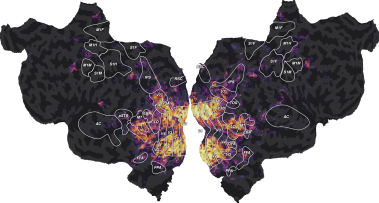
We can then plot the split scores on a flatmap with a 2D colormap.
from voxelwise_tutorials.viz import plot_2d_flatmap_from_mapper

mapper_file = os.path.join(directory, "mappers", f"{subject}_mappers.hdf")
ax = plot_2d_flatmap_from_mapper(split_scores[0], split_scores[1],
                                 mapper_file, vmin=0, vmax=0.25, vmin2=0,
                                 vmax2=0.5, label_1=feature_names[0],
                                 label_2=feature_names[1])
plt.show()
The blue regions are better predicted by the motion-energy features, the orange regions are better predicted by the wordnet features, and the white regions are well predicted by both feature spaces.
Compared to the last figure of the previous example, we see that most white regions have been replaced by either blue or orange regions. The banded ridge regression disentangled the two feature spaces in voxels where both feature spaces had good prediction accuracy (see previous example). For example, motion-energy features predict brain activity in early visual cortex, while wordnet features predict in semantic visual areas. For more discussions about these results, we refer the reader to the publications describing the banded ridge regression approach [Dupré la Tour et al., 2022, Nunez-Elizalde et al., 2019].
References#
T. Dupré la Tour, M. Eickenberg, A.O. Nunez-Elizalde, and J. L. Gallant. Feature-space selection with banded ridge regression. NeuroImage, 267:119728, 2022. doi:10.1016/j.neuroimage.2022.119728.
Trevor Hastie, Robert Tibshirani, and Jerome Friedman. The Elements of Statistical Learning. Springer New York, 2009.
A. Hsu, A. Borst, and F. E. Theunissen. Quantifying variability in neural responses and its application for the validation of model predictions. Network, 2004.
A. G. Huth, S. Nishimoto, A. T. Vu, T. Dupré la Tour, and J. L. Gallant. Gallant lab natural short clips 3t fMRI data. 2022. doi:10.12751/g-node.vy1zjd.
A. G. Huth, S. Nishimoto, A. T. Vu, and J. L. Gallant. A continuous semantic space describes the representation of thousands of object and action categories across the human brain. Neuron, 76(6):1210–1224, 2012.
S. Nishimoto, A. T. Vu, T. Naselaris, Y. Benjamini, B. Yu, and J. L. Gallant. Reconstructing visual experiences from brain activity evoked by natural movies. Current Biology, 21(19):1641–1646, 2011.
A. O. Nunez-Elizalde, A. G. Huth, and J. L. Gallant. Voxelwise encoding models with non-spherical multivariate normal priors. Neuroimage, 197:482–492, 2019.
M. Sahani and J. Linden. How linear are auditory cortical responses? Adv. Neural Inf. Process. Syst., 2002.
C. Saunders, A. Gammerman, and V. Vovk. Ridge regression learning algorithm in dual variables. 1998.
O. Schoppe, N. S. Harper, B. Willmore, A. King, and J. Schnupp. Measuring the performance of neural models. Front. Comput. Neurosci., 2016.