Visualize the hemodynamic response

In this example, we describe how the hemodynamic response function was estimated in the previous model. We fit the same ridge model as in the previous example, and further describe the need to delay the features in time to account for the delayed BOLD response.

Because of the temporal dynamics of neurovascular coupling, the recorded BOLD signal is delayed in time with respect to the stimulus. To account for this lag, we fit encoding models on delayed features. In this way, the linear regression model weighs each delayed feature separately and recovers the shape of the hemodynamic response function in each voxel separately. In turn, this method (also known as a Finite Impulse Response model, or FIR) maximizes the model prediction accuracy. With a repetition time of 2 seconds, we typically use 4 delays [1, 2, 3, 4] to cover the peak of the the hemodynamic response function. However, the optimal number of delays can vary depending on the experiment and the brain area of interest, so you should experiment with different delays.

In this example, we show that a model without delays performs far worse than a model with delays. We also show how to visualize the estimated hemodynamic response function (HRF) from a model with delays.

Path of the data directory

from voxelwise_tutorials.io import get_data_home

directory = get_data_home(dataset="shortclips")
print(directory)

/home/jlg/mvdoc/voxelwise_tutorials_data/shortclips

# modify to use another subject
subject = "S01"

Load the data

We first load and normalize the fMRI responses.

import os
import numpy as np
from scipy.stats import zscore
from voxelwise_tutorials.io import load_hdf5_array
from voxelwise_tutorials.utils import zscore_runs

file_name = os.path.join(directory, "responses", f"{subject}_responses.hdf")
Y_train = load_hdf5_array(file_name, key="Y_train")
Y_test = load_hdf5_array(file_name, key="Y_test")

print("(n_samples_train, n_voxels) =", Y_train.shape)
print("(n_repeats, n_samples_test, n_voxels) =", Y_test.shape)

# indice of first sample of each run
run_onsets = load_hdf5_array(file_name, key="run_onsets")

# zscore each training run separately
Y_train = zscore_runs(Y_train, run_onsets)
# zscore each test run separately
Y_test = zscore(Y_test, axis=1)

(n_samples_train, n_voxels) = (3600, 84038)
(n_repeats, n_samples_test, n_voxels) = (10, 270, 84038)

We average the test repeats, to remove the non-repeatable part of fMRI responses, and normalize the average across repeats.

Y_test = Y_test.mean(0)
Y_test = zscore(Y_test, axis=0)

print("(n_samples_test, n_voxels) =", Y_test.shape)

(n_samples_test, n_voxels) = (270, 84038)

We fill potential NaN (not-a-number) values with zeros.

Y_train = np.nan_to_num(Y_train)
Y_test = np.nan_to_num(Y_test)

Then, we load the semantic “wordnet” features.

feature_space = "wordnet"

file_name = os.path.join(directory, "features", f"{feature_space}.hdf")
X_train = load_hdf5_array(file_name, key="X_train")
X_test = load_hdf5_array(file_name, key="X_test")

print("(n_samples_train, n_features) =", X_train.shape)
print("(n_samples_test, n_features) =", X_test.shape)

(n_samples_train, n_features) = (3600, 1705)
(n_samples_test, n_features) = (270, 1705)

Define the cross-validation scheme

We define the same leave-one-run-out cross-validation split as in the previous example.

We define a cross-validation splitter, compatible with scikit-learn API.

from sklearn.model_selection import check_cv
from voxelwise_tutorials.utils import generate_leave_one_run_out

n_samples_train = X_train.shape[0]
cv = generate_leave_one_run_out(n_samples_train, run_onsets)
cv = check_cv(cv)  # copy the cross-validation splitter into a reusable list

Define the model

We define the same model as in the previous example. See the previous example for more details about the model definition.

from sklearn.pipeline import make_pipeline
from sklearn.preprocessing import StandardScaler
from voxelwise_tutorials.delayer import Delayer
from himalaya.kernel_ridge import KernelRidgeCV
from himalaya.ridge import RidgeCV
from himalaya.backend import set_backend

backend = set_backend("torch_cuda", on_error="warn")

X_train = X_train.astype("float32")
X_test = X_test.astype("float32")

alphas = np.logspace(1, 20, 20)

pipeline = make_pipeline(
    StandardScaler(with_mean=True, with_std=False),
    Delayer(delays=[1, 2, 3, 4]),
    KernelRidgeCV(
        alphas=alphas,
        cv=cv,
        solver_params=dict(
            n_targets_batch=500, n_alphas_batch=5, n_targets_batch_refit=100
        ),
    ),
)

from sklearn import set_config

set_config(display="diagram")  # requires scikit-learn 0.23
pipeline

Pipeline(steps=[('standardscaler', StandardScaler(with_std=False)),
                ('delayer', Delayer(delays=[1, 2, 3, 4])),
                ('kernelridgecv',
                 KernelRidgeCV(alphas=array([1.e+01, 1.e+02, 1.e+03, 1.e+04, 1.e+05, 1.e+06, 1.e+07, 1.e+08,
       1.e+09, 1.e+10, 1.e+11, 1.e+12, 1.e+13, 1.e+14, 1.e+15, 1.e+16,
       1.e+17, 1.e+18, 1.e+19, 1.e+20]),
                               cv=_CVIterableWrapper(cv=[(array([   0,    1, ..., 3598, 3599]), array..., (array([   0,    1, ..., 3598, 3599]), array([2400, 2401, ..., 2698, 2699])), (array([   0,    1, ..., 3298, 3299]), array([3300, 3301, ..., 3598, 3599])), (array([ 300,  301, ..., 3598, 3599]), array([  0,   1, ..., 298, ...301, ..., 598, 599])), (array([   0,    1, ..., 3598, 3599]), array([1800, 1801, ..., 2098, 2099]))]),
                               solver_params={'n_alphas_batch': 5,
                                              'n_targets_batch': 500,
                                              'n_targets_batch_refit': 100}))])

In a Jupyter environment, please rerun this cell to show the HTML representation or trust the notebook.
On GitHub, the HTML representation is unable to render, please try loading this page with nbviewer.org.

Fit the model

We fit on the train set, and score on the test set.

pipeline.fit(X_train, Y_train)

scores = pipeline.score(X_test, Y_test)
scores = backend.to_numpy(scores)
print("(n_voxels,) =", scores.shape)

(n_voxels,) = (84038,)

Understanding delays

To have an intuitive understanding of what we accomplish by delaying the features before model fitting, we will simulate one voxel and a single feature. We will then create a Delayer object (which was used in the previous pipeline) and visualize its effect on our single feature.

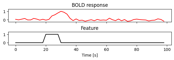
Let’s start by simulating the data. We assume a simple scenario in which an event in our experiment occurred at \(t = 20\) seconds and lasted for 10 seconds. For each timepoint, our simulated feature is a simple variable that indicates whether the event occurred or not.

from voxelwise_tutorials.delays_toy import create_voxel_data

# simulate an activation pulse at 20 s for 10 s of duration
simulated_X, simulated_Y, times = create_voxel_data(onset=20, duration=10)

We next plot the simulated data. In this toy example, we assumed a “canonical” hemodynamic response function (HRF) (a double gamma function). This is an idealized HRF that is often used in the literature to model the BOLD response. In practice, however, the HRF can vary significantly across brain areas.

Because of the HRF, notice that even though the event occurred at \(t = 20\) seconds, the BOLD response is delayed in time.

import matplotlib.pyplot as plt
from voxelwise_tutorials.delays_toy import plot_delays_toy

plot_delays_toy(simulated_X, simulated_Y, times)
plt.show()

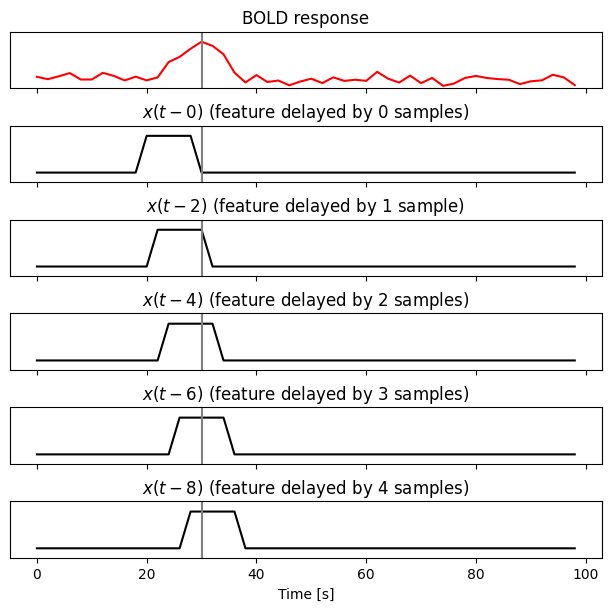
We next create a Delayer object and use it to delay the simulated feature. The effect of the delayer is clear: it creates multiple copies of the original feature shifted forward in time by how many samples we requested (in this case, from 0 to 4 samples, which correspond to 0, 2, 4, 6, and 8 s in time with a 2 s TR).

When these delayed features are used to fit a voxelwise encoding model, the brain response \(y\) at time \(t\) is simultaneously modeled by the feature \(x\) at times \(t-0, t-2, t-4, t-6, t-8\). For example, the time sample highlighted in the plot below (\(t = 30\) seconds) is modeled by the features at \(t = 30, 28, 26, 24, 22\) seconds.

# create a delayer object and delay the features
delayer = Delayer(delays=[0, 1, 2, 3, 4])
simulated_X_delayed = delayer.fit_transform(simulated_X[:, None])

# plot the simulated data and highlight t = 30
plot_delays_toy(simulated_X_delayed, simulated_Y, times, highlight=30)
plt.show()

This simple example shows how the delayed features take into account of the HRF. This approach is often referred to as a “finite impulse response” (FIR) model. By delaying the features, the regression model learns the weights for each voxel separately. Therefore, the FIR approach is able to adapt to the shape of the HRF in each voxel, without assuming a fixed canonical HRF shape. As we will see in the remaining of this notebook, this approach improves model prediction accuracy significantly.

Compare with a model without delays

We define here another model without feature delays (i.e. no Delayer). Because the BOLD signal is inherently slow due to the dynamics of neuro-vascular coupling, this model is unlikely to perform well.

Note that if we remove the feature delays, we will have more fMRI samples (3600) than number of features (1705). In this case, running a kernel version of ridge regression is computationally suboptimal. Thus, to create a model without delays we are using RidgeCV instead of KernelRidgeCV.

pipeline_no_delay = make_pipeline(
    StandardScaler(with_mean=True, with_std=False),
    RidgeCV(
        alphas=alphas,
        cv=cv,
        solver="svd",
        solver_params=dict(
            n_targets_batch=500, n_alphas_batch=5, n_targets_batch_refit=100
        ),
    ),
)
pipeline_no_delay

Pipeline(steps=[('standardscaler', StandardScaler(with_std=False)),
                ('ridgecv',
                 RidgeCV(alphas=array([1.e+01, 1.e+02, 1.e+03, 1.e+04, 1.e+05, 1.e+06, 1.e+07, 1.e+08,
       1.e+09, 1.e+10, 1.e+11, 1.e+12, 1.e+13, 1.e+14, 1.e+15, 1.e+16,
       1.e+17, 1.e+18, 1.e+19, 1.e+20]),
                         cv=_CVIterableWrapper(cv=[(array([   0,    1, ..., 3598, 3599]), array([600, 601, ..., 898, 899])), (array([   0,    1, ..., 3598, 3599]), array([2400, 2401, ..., 2698, 2699])), (array([   0,    1, ..., 3298, 3299]), array([3300, 3301, ..., 3598, 3599])), (array([ 300,  301, ..., 3598, 3599]), array([  0,   1, ..., 298, ...301, ..., 598, 599])), (array([   0,    1, ..., 3598, 3599]), array([1800, 1801, ..., 2098, 2099]))]),
                         solver_params={'n_alphas_batch': 5,
                                        'n_targets_batch': 500,
                                        'n_targets_batch_refit': 100}))])

In a Jupyter environment, please rerun this cell to show the HTML representation or trust the notebook.
On GitHub, the HTML representation is unable to render, please try loading this page with nbviewer.org.

We fit and score the model as the previous one.

pipeline_no_delay.fit(X_train, Y_train)
scores_no_delay = pipeline_no_delay.score(X_test, Y_test)
scores_no_delay = backend.to_numpy(scores_no_delay)
print("(n_voxels,) =", scores_no_delay.shape)

(n_voxels,) = (84038,)

Then, we plot the comparison of model prediction accuracies with a 2D histogram. All ~70k voxels are represented in this histogram, where the diagonal corresponds to identical prediction accuracy for both models. A distribution deviating from the diagonal means that one model has better prediction accuracy than the other.

from voxelwise_tutorials.viz import plot_hist2d

ax = plot_hist2d(scores_no_delay, scores)
ax.set(
    title="Generalization R2 scores",
    xlabel="model without delays",
    ylabel="model with delays",
)
plt.show()

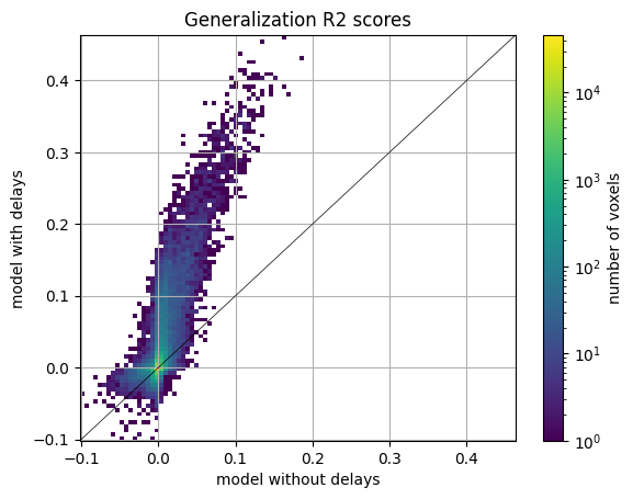
We see that the model with delays performs much better than the model without delays. This can be seen in voxels with scores above 0. The distribution of scores below zero is not very informative, since it corresponds to voxels with poor predictive performance anyway, and it only shows which model is overfitting the most.

Visualize the HRF

We just saw that delays are necessary to model BOLD responses. Here we show how the fitted ridge regression weights follow the hemodynamic response function (HRF).

Fitting a kernel ridge regression results in a set of coefficients called the “dual” coefficients \(w\). These coefficients differ from the “primal” coefficients \(\beta\) obtained with a ridge regression, but the primal coefficients can be computed from the dual coefficients using the training features \(X\):

(7)\[\begin{align}\beta = X^\top w\end{align}\]

To better visualize the HRF, we will refit a model with more delays, but only on a selection of voxels to speed up the computations.

# pick the 10 best voxels
voxel_selection = np.argsort(scores)[-10:]

# define a pipeline with more delays
pipeline_more_delays = make_pipeline(
    StandardScaler(with_mean=True, with_std=False),
    Delayer(delays=[0, 1, 2, 3, 4, 5, 6]),
    KernelRidgeCV(
        alphas=alphas,
        cv=cv,
        solver_params=dict(
            n_targets_batch=500, n_alphas_batch=5, n_targets_batch_refit=100
        ),
    ),
)

pipeline_more_delays.fit(X_train, Y_train[:, voxel_selection])

# get the (primal) ridge regression coefficients
primal_coef = pipeline_more_delays[-1].get_primal_coef()
primal_coef = backend.to_numpy(primal_coef)

# split the ridge coefficients per delays
delayer = pipeline_more_delays.named_steps["delayer"]
primal_coef_per_delay = delayer.reshape_by_delays(primal_coef, axis=0)
print("(n_delays, n_features, n_voxels) =", primal_coef_per_delay.shape)

# select the feature with the largest coefficients for each voxel
feature_selection = np.argmax(np.sum(np.abs(primal_coef_per_delay), axis=0), axis=0)
primal_coef_selection = primal_coef_per_delay[
    :, feature_selection, np.arange(len(voxel_selection))
]

plt.plot(delayer.delays, primal_coef_selection)
plt.xlabel("Delays")
plt.xticks(delayer.delays)
plt.ylabel("Ridge coefficients")
plt.title(f"Largest feature for the {len(voxel_selection)} best voxels")
plt.axhline(0, color="k", linewidth=0.5)
plt.show()

(n_delays, n_features, n_voxels) = (7, 1705, 10)

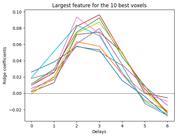
We see that the hemodynamic response function (HRF) is captured in the model weights. Note that in this dataset, the brain responses are recorded every two seconds.